MITRE at SemEval 2019 Task 5: Transfer Learning for Multilingual Hate Speech Detection

(1)

453

MITRE at SemEval-2019 Task 5: Transfer Learning for Multilingual

Hate Speech Detection

Abigail S. Gertner, John C. Henderson, Amy Marsh, Elizabeth M. Merkhofer, Ben Wellner and Guido Zarrella

The MITRE Corporation 202 Burlington Road Bedford, MA 01730-1420, USA

{gertner,jhndrsn,amarsh,emerkhofer,wellner,jzarrella}@mitre.org

Abstract

This paper describes MITRE’s participation in SemEval-2019 Task 5,HatEval: Multilin-gual detection of hate speech against immi-grants and women in Twitter. The techniques explored range from simple bag-of-ngrams classifiers to neural architectures with varied attention mechanisms. We describe several styles of transfer learning from auxiliary tasks, including a novel method for adapting pre-trained BERT models to Twitter data. Logis-tic regression ties the systems together into an ensemble submitted for evaluation. The result-ing system was used to produce predictions for all four HatEval subtasks, achieving the best mean rank of all teams that participated in all four conditions.

1 Introduction

The popularity of social media allows anyone to post their thoughts and opinions for all to see. While the vast majority of these communications are benign, there are those who express hateful or threatening messages online. The identification of hate speech (Fortuna and Nunes, 2018; Schmidt and Wiegand, 2017) on platforms like Twitter is of particular interest for law enforcement and to social media companies who wish to remove ac-counts with offending content from their sites. Au-tomating the identification of hate speech will al-low platforms to flag and remove content much more quickly and effectively.

In this effort we explored neural transfer learn-ing techniques, includlearn-ing word embeddlearn-ings and fine-tuning of models trained with diverse auxil-iary tasks. We built and compared models em-ploying soft attention over sequences and multi-headed self-attention. We also present a novel task to aid in performing additional pre-training of BERT (Devlin et al.,2018) for domain adaptation to Twitter data.

2 Task, Data and Evaluation

HatEval was a shared task organized within SemEval-2019 (Basile et al., 2019). The pri-mary task was detection of hate speech in Twit-ter, specifically against immigrants and women. This multilingual shared task was organized into two sub-tasks, each presented in both English and Spanish, for a total of four sub-task evaluations.

Task A The first sub-task was simply to identify tweets containing hate speech against immigrants or women. The official metric used for this binary classification task wasmacro-averaged F1 score, in which the F1 scores are calculated for both the positivehate speechand negativenot hate speech classes and then those two scores are averaged.

Task B The second sub-task involved the de-tection of two specific aspects of hate speech: whether it is targeted at an individual vs. a group of people, and whether it expresses aggression on the part of the author. In this annotation scheme, there is a dependency between these two cate-gories and the hate speech label used in Task A, as tweets could only be labeled as positive for tar-geting or aggression if they were positive for hate speech. The official metric used for Task B was Exact Match Ratio (EMR), which is the propor-tion of tweets that are labeled correctly for all cat-egories (hate speech, targeting, and aggression). Another way to think of this is as a five-class classification problem where the classes are (H=0, T=0, A=0), (H=1, T=0, A=0), (H=1, T=0, A=1), (H=1, T=1, A=0), (H=1, T=1, A=1). EMR on pre-dicting the three classes separately is equivalent to accuracy on this five-class classification.

(2)

Cursory examination revealed drastic differ-ences between the training and test sets, partic-ularly in English. The pejorative term bitch ap-peared in 12% of the training tweets vs. 48% of the test tweets. The hashtags #BuildThatWall or #BuildTheWallappeared at rates of 6% and 23% in train and test, respectively. Likewise,#MAGA was in over 12% of the test set tweets but in under 3% of the training set messages. Thus the English test set appears to be dominated by a handful of heavily represented phenomena.

Different annotation strategies appear to have been used on the training and test sets as well. While tweets mentioning#BuildThatWallor #BuildTheWallwere annotated as hate speech 98% of the time in the training set, this number is 35% on the test set. Similarly, tweets containingbitch were labeled as hate speech 78% of the time in the training set vs. 43% of the time in the test set.

The use of hashtags differs markedly between languages. Hashtags are much more frequent in the English training data than the Spanish training data, with English tweets 2.6 times more likely to contain at least one tag, and with tags occurring in English at 4.1 times the rate in Spanish. In the En-glish training data, the most frequent ten hashtags were 23% of the overall total and tended towards American political topics. In Spanish, the top ten tags account for only 8% of the total, exhibiting a much longer and sparser tail.

3 System Overview

For each task, we created an ensemble of systems, each of which independently predicted the classes. The component systems are described in the fol-lowing eight sections, after which we describe the procedure for building and testing the ensembles. All component systems described below treated Task B as a five-class prediction problem, and with the exception of two BERT-based systems, were trained to address Task A and Task B simultane-ously.

Data and resources SemEval organizers pro-vided training and development sets for English and Spanish. Planning to build ensembles, we shuffled and split out 10% of the training for cal-ibrating models in the ensembles (calibration set from here on). Components were trained using the remaining 90% of the training sets provided, with hyperparameter search and validation using the full development sets or via cross-validation.

We did not use any additional supervised datasets. The BiLSTM, Name Embedding, and Hash-tag Prediction models incorporated pre-trained

word2vec (Mikolov et al., 2013) language-specific embeddings that we trained on 1558 bil-lion English and 444 milbil-lion Spanish tweets col-lected from 2011 to 2018. In both cases we ap-pliedword2phrasetwice to identify phrases of up to four words, and trained a skip-gram model of size 256, using a context window of 10 words and 15 negative samples per example.

For Task A, all of our component systems and ensembles included a post-processing step to se-lect the best threshold score for classifying hate speech in order to achieve the maximum macro-averaged F1 score on the development set.

3.1 BiLSTM with Attention

We trained several heavily regularized single-layer Bidirectional LSTM (Hochreiter and Schmidhu-ber, 1997) models to learn a tweet representa-tion with soft attenrepresenta-tion (Bahdanau et al., 2014) over a sequence of pre-trained token embeddings. Hyperparameter experimentation with Spearmint (Snoek et al.,2012) suggested that a shallow net-work with attention outperformed deeper, stacked networks and networks without attention. Our at-tention layer learns to weight context-aware repre-sentations of each timestep of the input.

We trained one architecture for the English tasks and two architectures for Spanish, although the second was ablated from our Task A ensem-ble. The models were identical in structure and differed only in hyperparameters. All models were constructed with spatial dropout over a frozen em-bedding layer, followed by an emem-bedding trans-form, one bi-directional LSTM layer with dropout, an attention layer, and a fully-connected hidden layer with dropout.

In each of these models, the NLP representation was used as input to a small prediction network of latent predictions and residual connections de-scribed in Section3.5.

3.2 Name embeddings

This model added a name embedding input to our BiLSTM described above, in an effort to better model the demographics of the individuals ad-dressed within a tweet.

(3)

multiple usernames a single Twitter user had em-ployed during a multi-year longitudinal sample of random tweets streamed from the platform. This resulted in a vocabulary of approximately two mil-lion name pieces, which includes common names as well as alternate spellings using special charac-ters, symbols, emoji, and other text entered in the user namefield.

We extracted all substrings of at least length 3 from each username mention in a tweet and in-cluded any of them that were in our name embed-ding vocabulary as input to our model. We applied a learned transformation to each embedding and created a weighted combination with an attention layer. This was concatenated with a hidden repre-sentation constructed with the BiLSTM architec-ture described in Section3.1. This concatenation was the input to the prediction network described in Section3.5.

The Spanish name embedding was comprised of dropout over frozen embeddings, a dense em-bedding transform, and an attention layer. For En-glish, only an attention layer over the frozen em-beddings was used. The hyperparameters from our best English model were used in the BiLSTM ar-chitecture for both languages.

3.3 DeepMoji

The DeepMoji model developed by Felbo et al. (2017) predicts the emoji removed from an English-language tweet text. The authors train their RNN model on 1274 million tweets for a set of 64 emojis. Using varying degrees of fine-tuning and newly initialized layers, they test their distantly supervised models on several benchmark datasets for detecting emotion, sentiment, and sar-casm. The model’s best results used their chain-thaw fine-tuning method, which iteratively un-freezes and trains layers for the new objective. The authors distribute their trained model for the emoji prediction task.

We experimented with bothchain-thawtraining and models that were frozen until the final layer of abstraction in DeepMoji. The pre-trained model has a vocabulary that omits many of the hashtags and usernames that were important for our task. Our best model used 0.75 dropout over the output of a frozen DeepMoji model and three fully con-nected layers of sizes 512, 256, and 128 before the annotation constraint adapter. Chain thaw mod-els performed poorly and were ablated from our

Task A submission. DeepMoji models are only included in our English ensembles.

3.4 Hashtag prediction network

FollowingZarrella and Marsh (2016), we imple-mented a recurrent neural network classifier that was pre-trained via an auxiliary masked hashtag prediction task. We extracted 30 of the top hash-tags found in the training data, with 15 selected from both the hate speech positive and negative classes. Then we searched for the fifteen near-est neighbors of each tag via cosine similarity in embedding space, using vectors described in Sec-tion3. After removing duplicates, this resulted in 136 English and 132 Spanish hashtags. We down-loaded up to 1,000 recent tweets containing each hashtag from Twitter’s public search API, result-ing in 11,539 English tweets and 12,504 Spanish tweets. Tweets were stripped of the target hash-tag(s), and each corpus was divided into a training and development set using a 90/10 split.

The sequence of vector representations of the tokens in each tweet served as the input to a neu-ral network with a 128 LSTM units followed by a dense softmax layer over the possible candidate hashtags. Both the word embeddings and the re-current layer were tuned. These models correctly predicted development set hashtags with 50.3% accuracy on the English data and 56.6% accuracy on the Spanish data.

The trained weights were extracted from this network and used to initialize the five-way hate speech classifier for Task B, described in Sec-tion2, which additionally saw as input the one-hot representations of the 600 most frequent unigrams and 300 most frequent bigrams in the training data, each followed by a fully-connected dense layer. The size of each fully connected layer and amount of dropout were experimentally determined using Spearmint (Snoek et al.,2012) to maximize per-formance on the competition metrics on our de-velopment set.

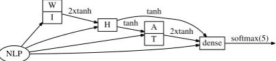
3.5 Annotation constraint adapter

(4)

NLP W

I

H A

T _dense 2xtanh

tanh tanh

2xtanh

[image:4.595.74.276.64.109.2]

softmax(5)

Figure 1: An annotation constraint adapter.

datasets, we believe they are latent variables that can be discovered in the NLP representation. Fig-ure 1 shows an adapter we placed at the end of several systems to encourage the network to learn these constraints. While it doesn’t enforce the con-straints, it sets up a principled graphical model that encourages the network to learn them. Of course, nothing prevents the network from learn-ing to model other thlearn-ings with this topology. Fair comparisons to stacked dense layers with the same number of parameters showed that the network with this topology performed better.

The upside to the design of a network like this is that the removal of the H switch might yield more general-purpose A and T classifiers.

3.6 Pre-training BERT with Twitter data

Pre-trained language models such as BERT (De-vlin et al., 2018) have been demonstrated to achieve state of the art performance on a range of language understanding tasks. BERT uses a trans-former encoder model (Vaswani et al.,2017) and pre-trains the model using two complementary ob-jectives: masked language model, and next sen-tence prediction. The pre-trained model may then be fine-tuned on labeled data (in this case the Hat-Eval dataset) to perform a downstream task.

For English, we used the BERT-Large model, which has 24 layers, 1024 hidden layer size, and 16 self-attention heads. For Spanish, we used the smaller multilingual BERT, with 12 layers, 768 hidden layer size, and 12 self-attention heads. The English BERT is trained on Wikipedia and BooksCorpus (Zhu et al.,2015), while the lingual model is trained on Wikipedia from multi-ple languages. As the language in these sources is likely to be quite different from the language com-monly used on Twitter, we elected to perform ad-ditional pre-training using a corpus of tweets col-lected during the same time period as the HatEval training dataset (October 2017 - September 2018). All of the pre-training experiments described be-low started from the TensorFbe-low model check-points downloaded from (Google Research,2018). Since the tweets in our collection are not

se-quential, they cannot be used for the next sen-tence prediction that BERT uses to learn sensen-tence relationships. We therefore began by running 20k steps of additional pre-training using only the masked language model task.

none MLM descriptions names

En A 79.1 81.2 79.7 NA

En B 66.4 69.0 67.9 NA

Es A 80.7 81.9 83.3 82.7

[image:4.595.316.517.140.197.2]

Es B 74.6 75.0 76.2 74.4

Table 1: Scores achieved with pre-training schemes. Due to time constraints, the name-based training was only done on Spanish models.

Next, we hypothesized that replacing the next-sentence prediction task with a task involving pre-dicting some attribute of the author of the tweet would provide the model with latent information about the nature of tweets that would allow it to discriminate between different classes of tweets more accurately. We performed 20k additional pre-training steps with the user description from the author’s Twitter profile standing in for the sec-ond sequence in the sentence prediction task. In other words, we trained the network to determine whether a given pair of (tweet text, author de-scription text) were sampled from the same tweet. Finally, we pre-trained a BERT model with the screen nameof the Twitter user as the secondary prediction task.

Table 1 shows the validation scores for our five-class model under our different pre-training schemes: No additional, pre-training on masked LM only, pre-training MLM + Twitter user descriptions, pre-training MLM + Twitter user screen names. Additional pre-training resulted in increased validation scores on all four tasks, and incorporating user descriptions in place of the next sentence prediction task further resulted in in-creased scores for both Spanish tasks.

3.7 Maximizing ensemble diversity

(5)

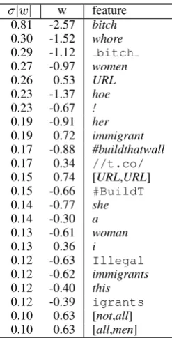
σ|w| w feature

0.81 -2.57 bitch

0.30 -1.52 whore

0.29 -1.12 bitch

0.27 -0.97 women

0.26 0.53 URL

0.23 -1.37 hoe

0.23 -0.67 !

0.19 -0.91 her

0.19 0.72 immigrant

0.17 -0.88 #buildthatwall

0.17 0.34 //t.co/

0.15 0.74 [URL,URL]

0.15 -0.66 #BuildT

0.14 -0.77 she

0.14 -0.30 a

0.13 -0.61 woman

0.13 0.36 i

0.12 -0.63 Illegal

0.12 -0.62 immigrants

0.12 -0.40 this

0.12 -0.39 igrants

[image:5.595.119.243.60.303.2]

0.10 0.63 [not,all] 0.10 0.63 [all,men]

Table 2: Top LRwordandcharacterfeatures.

BERT, using ensemble methods such as bagging directly proved too cumbersome as part of the model development workflow. Instead, we em-ployed a form of negative correlation learning (Liu and Yao, 1999) to train a small ensemble of neu-ral network classifiers within a single architecture. A term was added to the fine tuning cross entropy loss function which encouraged diversity among all pairs of classifiers followingOpitz et al.(2016).

3.8 Logistic Regression

Logistic regression (LR) systems were developed as a baseline against which the neural approach would be compared. Had annotators used very simple features such as words or phrases to make decisions, they would have been found in the course of LR training. Some of the systems were good enough to include in the final ensembles.

The vocabulary of the LR system was limited to the training set. Many feature sets were explored during model search. The best models preferred featuresetsrather thancountsorterm frequencies. Word n-grams of length 1-3 and character n-grams to length 8 were all considered, along with skip bigrams. The specifics of the best resulting fea-ture sets are in Table 3. Table2 shows the most important features from an English Task A LR system, sorted by feature influence, the product of feature function standard deviation and model weight. The second column is model weight, with negative weights contributing to a (H=1) decision.

In all cases, a bias term was added and

Liblinear(Fan et al.,2008) was used to com-pute the model. L2 regularization was used to en-courage generalization. Cross-validation was used to pick the regularization parameters.

3.9 Ensemble

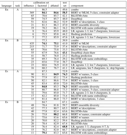
Many systems were created, and final ensembles were constructed by incremental ablations. An ini-tialall-inensemble was created and tested, then it was tested with each component removed. This process was iterated on the best performing ab-lated sets until gains were no longer observed. Ap-proximately two thousand total ensembles were created through the ablative search. Two systems were ablated in Task A EN, three in Task A ES, one in both Task B conditions. Those systems are not described in this paper.

Ensembles were constructed using logistic re-gression on either the classifier outputs or the classifier outputs and final probabilities from the model. One oddity to note is that the ensembles using the probabilities performed better for Task A and the ensembles ignoring the probabilities per-formed better in Task B.

Table3shows ensemble compositions for each of the four tested conditions. The first column, labeled influence, indicates the influence that the particular component has on the ensemble. It is the number of cases in which that component’s contri-butionchangesthe outcome of the ensemble. It is calculated by zeroing out all LR weights for that particular component and noting the difference. In English, the BERT models had the most influence, while in Spanish, the influence was more evenly distributed across the components.

4 Results

Table 3 shows performance of our component models and ensembles. The calibration set fac-toredcolumn shows the performance of the com-ponent on our calibration data. This is themacro averaged F1 score for Task A and Exact Match Ratiofor Task B. Thecalibration set ablated col-umn shows the performance of the ensemble when that component is removed and the ensemble pa-rameters are re-optimized. Finally there are the scores we calculated after the evaluation period for each of our components using the released refer-ence sets.

(6)

calibration set test

language task influence factored ablated set component

En A 86.5 49.6 combo

369 84.1 84.6 58.5 BERT w/ MLM, 5-class, constraint adapter

65 78.6 85.7 42.1 BiLSTM+Attn

59 74.5 85.7 48.0 DeepMoji

51 82.6 86.2 52.9 BERT w/ descriptions, 1-class

21 81.3 86.3 47.0 BERT ensemble diversity

19 78.2 86.1 34.2 BiLSTM with name embeddings

8 76.4 85.9 48.0 LR, ngrams 1-3, len 7 chargrams, lowercase

6 75.5 85.8 44.2 Hashtag prediction

En B 77.3 39.9 combo

435 74.1 75.1 41.0 BERT w/ MLM

215 71.7 75.9 37.4 BERT w/ descriptions, constraint adapter

65 70.6 75.8 33.3 BiLSTM+Attn

55 67.9 76.6 43.1 DeepMoji chain-thaw

23 65.6 77.0 38.7 DeepMoji

16 68.2 76.7 41.1 LR, unigrams, len 5 chargrams, lc, skip bigrams

Es A 87.3 72.9 combo

90 81.1 84.9 74.3 BERT w/ names, 5-class

50 82.1 86.6 73.4 BERT w/ names, 1-class

45 83.4 85.0 72.0 BiLSTM+Attn

35 80.7 86.8 73.3 BERT w/ names, 5-class, constraint adapter

32 79.6 85.0 71.7 LR, ngrams 2-3, len 4 chargrams, lc

15 81.4 86.0 73.7 BERT w/ descriptions, 1-class

Es B 84.7 67.1 combo

42 77.3 80.7 65.3 BERT w/ descriptions

40 77.8 82.4 63.6 BiLSTM+Attn

26 75.8 80.2 66.8 BERT w/ names, constraint adapter

21 75.6 83.6 65.6 BERT w/ names

20 70.0 82.2 59.4 Hashtag predictions

20 78.4 82.9 67.4 BiLSTM+Attn

19 76.4 82.4 68.8 LR, ngrams 1-3, chargrams 4-7, lc

15 76.2 82.0 66.7 BERT w/ descriptions, constraint adapter

[image:6.595.95.506.59.497.2]

Table 3: Ensembles and Components

are 49.6% and 72.9% Macro F1 on HatEval Task A English and Spanish, respectively, and 39.9% and 67.1% EMR on Task B English and Spanish. A full reporting of results is present inBasile et al. (2019). A breakdown of test results shows that our system achieves hate speech detection F1 of 63.9 and 72.7 in English and Spanish, respectively, which ranked 2nd (of 68) and 1st (of 39) within Task A. The rankings within Task B were similar, with mean macro F1 of 61.4 and 77.2 in English and Spanish, respectively, ranking 2nd (of 42) and 1st (of 24). Finally, we note that only 22 out of the 74 participants submitted entries in all four sub-tasks. Of those 22 teams, these results represent the top mean rank across all subtasks.

5 Conclusion

An ensemble of models was used to classify tweets according to whether they contained hate speech, aggression, and targeting of individuals. The novel contributions include using name embed-dings, substituting twitter author profile prediction for next sentence prediction in BERT pre-training, and augmenting BERT’s fine-tuning loss function with a diversity term to create an ensemble.

There is a discrepancy between the official test set results and our held-out calibration set, partic-ularly in the English subtasks, which we attribute to dataset divergences like those called out in Sec-tion2.

(7)

References

Dzmitry Bahdanau, Kyunghyun Cho, and Yoshua Ben-gio. 2014. Neural machine translation by jointly learning to align and translate. InInternational Con-ference on Learning Representations Workshop.

Valerio Basile, Cristina Bosco, Elisabetta Fersini, Deb-ora Nozza, Viviana Patti, Francisco Rangel, Paolo Rosso, and Manuela Sanguinetti. 2019. SemEval-2019 task 5: Multilingual detection of hate speech against immigrants and women in Twitter. In Pro-ceedings of the 13th International Workshop on Se-mantic Evaluation (SemEval-2019).

Leo Breiman. 1996. Bagging predictors. Machine learning, 24(2).

Jacob Devlin, Ming-Wei Chang, Kenton Lee, and Kristina Toutanova. 2018. Bert: Pre-training of deep bidirectional transformers for language understand-ing. arXiv preprint arXiv:1810.04805.

Rong-En Fan, Kai-Wei Chang, Cho-Jui Hsieh, Xiang-Rui Wang, and Chih-Jen Lin. 2008. LIBLINEAR: A library for large linear classification. Journal of Machine Learning Research, 9:1871–1874.

Bjarke Felbo, Alan Mislove, Anders Søgaard, Iyad Rahwan, and Sune Lehmann. 2017. Using millions of emoji occurrences to learn any-domain represen-tations for detecting sentiment, emotion and sar-casm. InConference on Empirical Methods in Nat-ural Language Processing (EMNLP).

Paula Fortuna and S´ergio Nunes. 2018. A survey on automatic detection of hate speech in text. ACM Comput. Surv., 51(4):85:1–85:30.

Google Research. 2018. https://github.com/

google-research/bert.

Sepp Hochreiter and J¨urgen Schmidhuber. 1997. Long short-term memory. Neural computation, 9(8):1735–1780.

Yong Liu and Xin Yao. 1999. Ensemble learn-ing via negative correlation. Neural networks, 12(10):1399–1404.

Tomas Mikolov, Ilya Sutskever, Kai Chen, Greg S Cor-rado, and Jeff Dean. 2013. Distributed representa-tions of words and phrases and their compositional-ity. InAdvances in Neural Information Processing Systems.

Michael Opitz, Horst Possegger, and Horst Bischof. 2016. Efficient model averaging for deep neural net-works. InAsian Conference on Computer Vision.

Anna Schmidt and Michael Wiegand. 2017. A survey on hate speech detection using natural language pro-cessing. In Proceedings of the Fifth International Workshop on Natural Language Processing for So-cial Media.

Jasper Snoek, Hugo Larochelle, and Ryan P Adams. 2012. Practical bayesian optimization of machine learning algorithms. InAdvances in neural informa-tion processing systems.

Ashish Vaswani, Noam Shazeer, Niki Parmar, Jakob Uszkoreit, Llion Jones, Aidan N Gomez, Łukasz Kaiser, and Illia Polosukhin. 2017. Attention is all you need. InAdvances in Neural Information Pro-cessing Systems.

Guido Zarrella and Amy Marsh. 2016. MITRE at SemEval-2016 task 6: Transfer learning for stance detection. InSemEval@NAACL-HLT.