Modeling language evolution
with codes that utilize context and phonetic features
Javad Nouri and Roman Yangarber Department of Computer Science
University of Helsinki, Finland
Abstract
We present methods for investigating pro-cesses of evolution in a language fam-ily by modeling relationships among the observed languages. The models aim to find regularities—regular correspon-dences in lexical data. We present an al-gorithm which codes the data using pho-netic features of sounds, and learns long-range contextual rules that condition re-current sound correspondences between languages. This gives us a measure of model quality: better models find more regularity in the data. We also present a procedure for imputing unseen data, which provides another method of model com-parison. Our experiments demonstrate im-provements in performance compared to prior work.
1 Introduction
We present work on modeling evolution within language families, by discovering regularity in data from observed languages.
The study of evolution of language families covers several problems, including: a. discovering
cognates—“genetically related” words, i.e., words
that derive from a common ancestor word in an ancestral proto-language; b. determining genetic relationships among languages in the given lan-guage family based on observed data; c. discover-ing patterns of sound correspondence across lan-guages; and d. reconstruction of forms in proto-languages. In this paper, we treat a. (sets of cog-nates) as given, and focus on problems b. and c.1
Given a corpus of cognate sets,2 we first aim to
1Extending the methods to problem d. is future work. 2The members of a cognate set are posited (by linguists)
to derive from a common, shared origin: a word-form in the (typically unobserved) ancestral proto-language.
find as much regularity as possible in the data at the sound (or symbol) level.3An important goal is that our methods be data-driven—we aim to use all data available, and to learn the patterns of regular correspondence directly from the data. We allow only the data to determine which rules underlie it—correspondences that are inherently encoded
in the corpus itself—rather than relying on exter-nally supplied (and possibly biased) rules or “pri-ors.” We try to refrain froma prioriassumptions or “universal” principles—e.g., no preference to align consonants with consonants, to align a sym-bol with itself, etc.
We claim that alignment may not be the best way to address the problem of regularity. Finding alignments is indeed finding a kind of regularity, but not all regularity is expressed as alignment.
The paper is organized as follows. In section 2 we review the data used in our experiments and re-cent approaches to modeling language evolution. We formalize the problem and present our mod-els in section 3. The modmod-els treat sounds as vec-tors of phoneticfeatures, and utilize thecontextof the sounds to discover patterns of regular corre-spondence. Once we have obtained the regularity, the question arises how we can evaluate it effec-tively. In section 4, we present a procedure for imputation—prediction of unseen data—to evalu-ate the strength of the learned rules of correspon-dence, by how well they predict words in one guage given corresponding words in another lan-guage. We further evaluate the models by using them for building phylogenies—family trees, and comparing them to gold standards, in section 4.2. We conclude with a discussion in section 5.
We have experimented with several language families: Uralic, Turkic and Indo-European; the paper focuses on results from the Uralic family.
3NB: we usesoundsandsymbolsinterchangeably, as we
assume that input data is rendered in a phonetic transcription.
We use large-scale digital etymological re-sources/dictionaries. For Uralic, the StarLing database, (Starostin, 2005), contains 2586 Uralic cognate sets, based on (R´edei, 1991). The et-ymological dictionarySuomen Sanojen Alkuper¨a
(SSA), “The Origin of Finnish Words,” (Itkonen and Kulonen, 2000), has over 5000 cognate sets.
2 Related work and motivation
One traditional arrangement of the Uralic lan-guages is shown in Figure 1; several alternative arrangements appear in the literature.
The last 15 years have seen a surge in computa-tional modeling of language relationships, change and evolution. We provide a detailed discussion of related prior work in (Nouri et al., 2016).
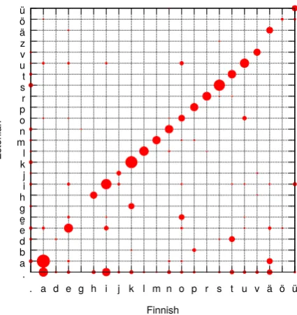
In earlier work, e.g., (Wettig et al., 2011), we presented two perspectives on the problem of find-ing regularity. It can be seen as a problem of align-ing the data. From an information-theoretic per-spective, finding regularity is a problem of com-pression: the more regularity we find in data, the more we can compress it. In (Wettig et al., 2011), we presented baseline models, which fo-cus on alignment of symbols, in a 1-1 fashion. We showed that aligning more than one symbol at a time—e.g., 2-2—gives better performance. Alignment is a natural way to think of comparing languages. E.g., in Figure 2, obtained by the 1-1 model, we can observe4 that most of the time Finnish k corresponds to Estonian k (we write Fin. k ∼ Est. k). However, models that focus on alignments have certain shortcomings. For ex-ample, substantial probability mass is assigned to Fin.k∼Est.g, yet the model cannot explain why. Fin.k ∼Est.g in certain environments—in non-first syllables, between vowels or after a voiced consonant—but the model cannot capture this reg-ularity, because it has no notion ofcontext. In fact, the regularity is much deeper: not only Fin.k, but all Finnish voiceless stops become voiced in Esto-nian in this environment:p ∼b,t∼d. This type of regularity cannot be captured by the baseline model because it treats symbols as atoms, and does not know about their shared phonetic features.
We claim that alignment may always not be the best way to think about the problem of finding reg-ularity. Figure 2 shows a prominent “diagonal,”
4The size of the circle is proportional to the probability
of aligning the corresponding symbols on the X and Y axes. Thedotcoordinates “.” correspond to deletions/insertions.
. a b d e e̮
g hi j kl mn o pr st uv z ä ö ü
. a d e g h i j k l m n o p r s t u v ä ö ü
Estonian
[image:2.595.312.525.60.286.2]Finnish
Figure 2: 1-1 alignment for Finnish and Estonian
many sounds correspond—they “align with them-selves.” However, as languages diverge further, this correspondence becomes blurry; e.g., when we try to align Finnish and Hungarian, the prob-ability distribution of aligned symbols has much higher entropy, Figure 3. The reason is that the regularity lies on a much deeper level: predict-ing which sound occurs in a given position in a word requires knowledge of a wider context, in both Finnish and Hungarian. Hence we will prefer to think in terms ofcoding, rather than alignment. Methods in (Kondrak, 2002), learn one-to-one sound correspondences between words in pairs of languages. Kondrak (2003), Wettig et al. (2011) find more complex—many-to-many— correspondences. These methods focus on align-ment, and modelcontextof the sound changes in a limited way, while it is known that most evolu-tionary changes are conditioned on the context of the evolving sound. Bouchard-Cˆot´e et al. (2007) use MCMC-based methods to model context, and operate on more than a pair of languages.5
Our models, similarly to other work, operate at the phonetic level only, leaving semantic judge-ments to the creators of the database. Some prior work attempts to approach semantics by com-putational means as well, e.g., (Kondrak, 2004; Kessler, 2001). We begin with a set of etymo-logical data for a language family as given, and treat each cognate set as a fundamental unit of
in-5The running time did not scale well when the number of
Uralic
Samoyedic
South Samoyedic
Sayan Samoyedic
Kamas Karagas
Koibal Motor Soyot Taigi Selkup North Samoyedic
Nganasan Enets
Nenets Finno-Ugric
Ugric
Hungarian Ob-Ugric
Khanty Mansi Finnic
Permic
Komi Udmurt Mari West Finnic
Mordvin North Finnic
Sami Baltic Finnic
Finnish
Estonian Figure 1: Uralic language family (adapted from Encyclopedia Britannica)
. a b d d́
ef g hi j kl mn o pr st uv z ö ü
āč ēī ĺ ń ōš ū ǖ
ȫ
. a d e h i j k l m n o p r s t u v ä ö ü
Hungarian
[image:3.595.73.525.60.225.2]Finnish
Figure 3: 1-1 alignment for Finnish and Hungarian
put. We use the principle ofrecurrent sound
cor-respondence, as in much of the literature.
Alignment can be evaluated by measuring rela-tionships among entire languages within the fam-ily. Construction of phylogenies is studied, e.g., in (Nakhleh et al., 2005; Ringe et al., 2002; Barbanc¸on et al., 2009).
Our work is related to the generative “Berkeley” models, (Bouchard-Cˆot´e et al., 2007), (Hall and Klein, 2011), in the following respects.
Context: in (Wettig et al., 2011) we capture
some context by coding pairs of symbols, as in (Kondrak, 2003). Berkeley models handle con-text by conditioning the symbol being generated upon the immediately preceding and following symbols. Our method uses broader context by
building decision trees, so that non-relevant con-text information does not grow model complexity.
Phonetic features: in (Wettig et al., 2011) we
treated sounds/symbols as atomic—not analyzed in terms of their phonetic makeup. Berkeley mod-els use “natural classes” to define the context of a sound change, but not to generate the symbols themselves; (Bouchard-Cˆot´e et al., 2009) encode as a prior which sounds are “similar” to each other. We code symbols in terms of phonetic features. Our models are based on information-theoretic Minimum Description Length principle (MDL), e.g., (Gr¨unwald, 2007)—unlike Berkeley. MDL brings some theoretical benefits, since mod-els chosen in this way are guided by data with no free parameters or hand-picked “priors.” The data analyst chooses the model class and structure, and the coding scheme, i.e., a decodable way to en-code model and data. This determines the learning strategy—we optimize the cost function, which is the code length determined by these choices.
Objective function: we use NML—the
normal-ized maximum likelihood, not reported previously in this setting. It is preferable for theoretical and practical reasons, e.g., to prequential coding used in (Wettig et al., 2011), as explained in section 3.1. Models that utilize more than the immediate ad-jacent environment of a sound to build a complete alignment of a language family have not been re-ported previously, to the best of our knowledge.
3 Coding pairs of words
[image:3.595.77.287.245.505.2]sym-bols correspond best; the task of coding is achiev-ing more compression. The simplest form of sym-bol alignment is a pair(σ :τ) ∈ Σ×T, a single symbolσfrom thesource alphabetΣwith a sym-bolτ from thetarget alphabetT.
To modelinsertionsanddeletions, we augment both alphabets with a special “empty” symbol— denoted by a dot—and write the augmented alphabets asΣ. andT.. We can then align word pairs, such as hiiri—l¨oNk@r (meaning “mouse”
in Finnish and Khanty) in many different ways; putting Finnish (source level, above) and Khanty (target level, below), for example:
[image:4.595.328.501.62.171.2]h i . . i r i
| | | | | | |
l ¨o N k @ r .
. h . . i i r i
| | | | | | | |
l ¨o N k @ r . .
...
A final note about alignments: we find no satis-factory way toevaluatealignments. Which of the above alignments is “better”? It may be satisfying to prefer the left one, observing that Fin.h corre-sponds well to Khn.l(since they both go back to Proto-Uralicˇs); Fin. r ∼ Khn. r, etc. However,
if a model achieves better compression by prefer-ring the alignment on the right, then it is difficult to argue that that alignment is “not correct.”
3.1 Context model with phonetic features
Our coding method is based on MDL. The most refined form of MDL, NML—Normalized Maxi-mum Likelihood, (Rissanen, 1996)—cannot be ef-ficiently computed for our model. Therefore, we resort to a classic two-part coding scheme. The first part of the two-part code is responsible for splitting the data into subsets corresponding to cer-tain contexts. However, given the contexts, wecan
use NML to encode these subsets.6
We begin with a raw set of observed data— word pairs in two languages. We search for a way to code the data, by capturing regular correspon-dences. The goodness of the code is defined for-mally below. MDL says that the more regularity we can find in the data, the fewer bits we will need to encode (or compress) it. More regularity means lower entropy in the distribution that describes the data, and lower entropy lets us construct a more economical code.
Features:Rather than coding symbols (sounds) as atomic, we code them in terms of their
pho-6Theoretical benefits of NML over other coding
schemes include freedom from priors, invariance to re-parametrization, and other optimality properties, which are outside the scope of this paper, (Rissanen, 1996).
Context model
j a l k a
j a l g
[ ζ χ φ ψ ] [ α β γ δ ]
[ ξ π μ ω ]
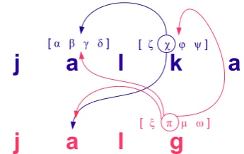
Figure 4: Fin.jalka(source)∼Est.jalg(target)
netic features. For example, figure 4 shows how a model might code Finnishjalkaand Estonianjalg
(meaning “leg”). We code the symbols in a fixed order: top to bottom, left to right. Each symbol is coded as a vector of its phonetic features, e.g., k= [ξ χ φ ψ].
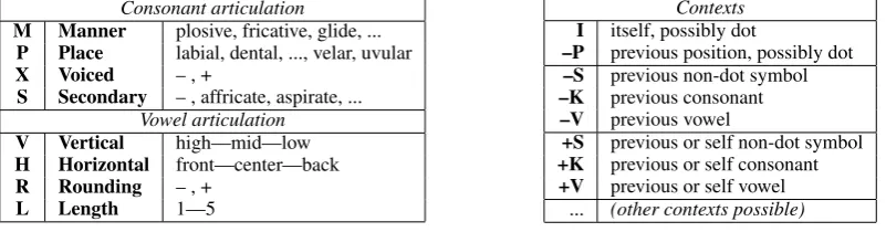
For each symbol, first we code a special Type
feature, with values: K (consonant), V (vowel), dot (insertion / deletion), or#(word boundary).7 Consonants and vowels have different sets of fea-tures; each feature has 2–8 values, listed in Fig-ure 5A. FeatFig-ures are coded in a fixed order.
Contexts: While coding each feature of the symbol, the model is allowed to query a fixed and finite a set ofcandidate contexts. The idea is that the model can query its “history”—information that has already been coded previously. When coding k, e.g., the model may query features of bluea(β, γ, etc.), as well as features of reda, etc. When codinggthe model may query those, and in addition also the features ofk(χ, φ, etc.)
Formally, a context is a triplet (L, P, F): Lis the level—source (σ) or target (τ); P is one of the positions that the model may query—relative to the position currently being coded; for example, we may query positions shown in Figure 5B.F is one of the possible features found at that position. Thus, we have in total about 2 levels×8 positions
×5 features≈80 candidate contexts that can be queried, as explained in detail below.
3.2 Two-part code
We code the complete (i.e., aligned) data using a two-part code, following MDL. We first code which model instance we select from our model
class, and then code the data given the model. Our
model class is defined as follows: a set of decision trees (forest)—one tree per feature per level (
sepa-ratelyfor source and for target). A modelinstance
Consonant articulation
M Manner plosive, fricative, glide, ...
P Place labial, dental, ..., velar, uvular
X Voiced – , +
S Secondary – , affricate, aspirate, ...
Vowel articulation
V Vertical high—mid—low
H Horizontal front—center—back
R Rounding – , +
L Length 1—5
Contexts
I itself, possibly dot
–P previous position, possibly dot –S previous non-dot symbol –K previous consonant –V previous vowel
+S previous or self non-dot symbol +K previous or self consonant +V previous or self vowel
... (other contexts possible) Figure 5: (A: left) Phonetic features and (B: right) phonetic contexts / environments.
will define a particular structure for each tree.
Cost of coding the structure: Thus, the forest consists of18decision trees—one for each feature on the source and the target level: the type feature, 4vowel and4consonant features, times 2levels. Each node in a tree will either be a leaf, or will be split—by querying one of the candidate con-texts defined above. The cost of a tree is one bit for every nodeni—to encode whetherni is nal (was split) or a leaf—plus the number of inter-nal nodes× ≈log 80—to encodewhichparticular context was chosen to split each ni. We explain how the model chooses the best candidate context on which to split a node in section 3.3.
Each feature and level define a tree, e.g., the “voiced” (X) feature of the source symbols— corresponds to the σ-X tree. A node N in this tree holds a distribution over the values of fea-tureXof only those symbol instances in the com-plete data that have reached node N, by follow-ing the context queries from the root downward. The tree structure tells us precisely which path to follow—completely determined by the context. When coding a symbolα based on another sym-bol found in the context C of α—for example, C = (τ,−K,M): at levelτ, position –K, and one of the features M—the next edge down the tree is determined by that feature’s value; and so on, down to a leaf.8
Cost of the data given the model: is computed by taking into account only the distributions atthe
leaves. The code will assign a cost (code-length)
to every possible alignment of the data. The total code-length is theobjectivefunction that the learn-ing algorithm will optimize.
Coding scheme:we use Normalized Maximum Likelihood (NML), and prequential coding as in (Wettig et al., 2011). We code the distribution at
8Model code to construct trees from data, and examples of
decision trees learned by the model are made publicly avail-able on the Project Web site:etymon.cs.helsinki.fi/.
each leaf node separately; the sum of the costs of all leaves gives the total cost of the complete data—the value of the objective function.
Supposeninstances reach a leaf nodeN, of the tree for feature F on level λ, and F has k val-ues: e.g.,nconsonants satisfyingN’s context con-straints in theσ-Xtree, withk= 2values:{−,+}. Suppose also that the values are distributed so that ni instances have value i, with i ∈ {1, . . . , k}. Then this requires an NML code-length of:
LNML(λ;F;N) =−logPNML(λ;F;N) =−log
Q i nni
ni
C(n, k) (1) HereQi ni
n ni
is the maximum likelihood of the multinomial data at nodeN, and the term
C(n, k) = X n0
1+...+n0k=n
Y
i
n0
i n
n0
i
(2)
is a normalizing constant to makePNMLa proba-bility distribution. In MDL literature, (Gr¨unwald, 2007), the term −logC(n, k) is called the
para-metric complexity or the (minimax) regret of the
model—in this case, the multinomial model. The NML distribution is the unique solution to the mini-max problem posed in (Shtarkov, 1987),
min ˆ
P maxxn log
P(xn|Θˆ(xn)) ˆ
P(xn) (3) where ˆΘ(xn) = arg max
ΘP(xn) are the
maxi-mum likelihood parametersfor the dataxn. Thus,
PNML minimizes the worst-case regret, i.e., the number of excess bits in the code as compared to the best model in the model class, with hind-sight. Details on the computation of this code length are given in (Kontkanen and Myllym¨aki, 2007).
[image:5.595.89.490.64.169.2]trees so as to minimize the two-part code length: the sum of the model’s code length—encoding the structure of the trees,—and the code length of the data given the model—encoding the aligned word pairs using these trees.
Summary of the algorithm: We start with an initialrandomalignment for each pair of words in the corpus. We then alternate between two steps:
A. re-build the decision trees for all features on source and target levels, and B.re-align all word pairs in the corpus, using dynamic programming. Both of these operations monotonically decrease the two-part cost function and thus compress the data. We continue until we reach convergence.
Simulated annealing with a slow cooling sched-ule is used to avoid getting trapped in local optima.
3.3 Building decision trees
Given a complete alignment of the data, we need to build a decision tree, for each feature on both levels, yielding the lowest two-part cost.The term “decision tree” is meant in a probabilistic sense: at each node we store a distribution over the re-spective feature values, for all instances that reach this node. The distribution at a given leaf is then used to code an instance when it reaches the leaf. We code the features in a fixed, pre-set order, and source level (σ-level) before target (τ-level).
We now describe in detail the process of build-ing the tree—usbuild-ing as example a tree for the σ-level feature X. (We will need do the same for all other features, on both levels, as well.) First, we collect all instances of consonants onσ-level, gather the the counts for feature X, and build an initial count vector; suppose it is:
value ofX→ + – 1001 1002
This vector is stored at the root of the tree; the cost of this node is computed using NML, eq. 1. Note that this vector / distribution has rather high entropy.
Next, we try to split this node, by finding such a context that if we query the values of the feature in that context, it will help us reduce the entropy in this count vector. We check in turn all possi-ble candidate contexts(L, P, F), and choose the best one. Each candidate refers to some symbol found onσ-level orτ-level, at some relative posi-tionP, and to one of that symbol’s featuresF. We will condition the split on the possible values ofF. For each candidate, we try to split on its feature’s
values, and collect the resulting alignment counts. Suppose one such candidate is (σ, –V,H), i.e., (σ-level, previous vowel, Horizontal feature), and suppose that theH-feature has two values: front / back. Suppose also that the vector at the root node (recall, this tree is for the X-feature) would then split into two vectors, for example:
value ofX→ + –
X|H=front 1000 1
X|H=back 1 1001
This would likely be a very good split, since it reduces the entropy of the distribution in each row to near zero. The criterion that guides the choice of the best candidate context to use for splitting a node is thesumof the code lengths of the resulting split vectors, and the code length is proportional to the entropy.
We go through all candidates exhaustively,9and greedily choose the one that yields the greatest re-duction in entropy, and drop in cost. We proceed recursively down the tree, trying to split nodes, and stop when the total tree cost stops decreasing. This completes the tree for featureXon levelσ. We build all remaining trees—for all features and all levels similarly—based on the current align-ment of the complete data.
3.4 Variations of context-based models
The context models enable us to discover more regularities in the data by querying the context of sounds. However building decision trees repeat-edly in the process of searching for the optimal alignments is very time consuming. We have ex-plored several variations of context-based models in an attempt to make the search converge more quickly, without sacrificing quality.
3.4.1 Zero-depth context model
In this variant of the model, during the simulated annealing phase (i.e., when there is some random-ness in the search algorithm), the trees are not ex-panded to their full depth. Instead, for source-level trees, only the root node is calculated and the tar-get level trees are allowed to query only theitself
position on the source level. Once the simulated annealing reaches the greedy phase, the trees are
9We augment the set of possible feature values at every
grown in the same way as they would have been normally, without any restrictions.
This model results in reasonable alignments and relatively low costs and lower running time.
3.4.2 Infinite-depth context model
This is another restrictive variation of the context model, which is more permissive than the zero-depth model. In this variation during the simulated annealing phase of the algorithm, the candidates that can be queried to expand the root nodes of the trees are limited to already encoded features of the
itselfposition.
4 Evaluation
We discuss two views on evaluation—strict evalu-ations vs.intuitiveevaluations.
4.1 Comparing context models to each other
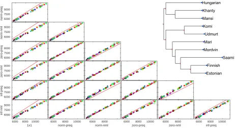
From a strictly information-theoretic point of view, a sufficient condition to claim that modelM1 is better thanM2, is thatM1assigns a higher prob-ability (equivalently—lower cost) to the observed data. Figure 7A shows the absolute costs,in bits, for all language pairs—for the baseline 1-1 model and six context models. The six context models are: the “normal” model, zero-depth and infinite-depth—and for each, the objective function uses either NML or prequential coding.
Here is how we interpret the points in these scat-ter plots. Each box in the triangular plot com-pares one model, Mx—whose scores are plotted on the X-axis—against another model,My(on the Y-axis). For example, the leftmost column com-pares the baseline 1-1 model as Mx against each of the six context models in turn; etc. In every plot box, each of the10×9points is a comparison of the two modelsMxandMy on one language pair (L1, L2). Therefore, for each point(L1, L2), the X-coordinate gives the score of modelMx, and the Y-coordinate gives the score of the other model, My. If the point (L1, L2) is below the diagonal, Mxhas higher cost on(L1, L2)thanMy. The fur-ther away the point is from the “break-even” diag-onal linex = y, the greater the advantage of one model over the other.
The left column of figure 7A shows that all con-text models always produce much lower cost com-pared to the basic context-free 1-1 model defined in (Wettig et al., 2011).
The remaining five columns compare the con-text models among themselves. Here we see that
0 20 40 60 80 100 120 140 160
0 500 1000 1500 2000 2500 3000 3500
Compressed size x1000 bits
[image:7.595.309.534.63.226.2]Data size: number of word pairs (average word-length: 5.5 bytes) Gzip Bzip2 1-1 model 2-2 model Context model
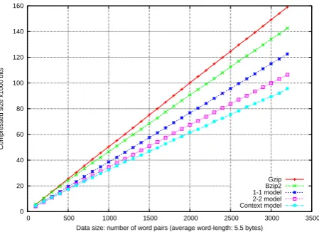
Figure 6: Comparison of compression power
no model variant is a clear winner. Since the vari-ants do not show a clear preference for the “best” context model among this set, we will use all of them, to vote as an ensemble.
In figure 6, we compare the context model against standard data compressors, Gzip and Bzip, as well as the baseline models in (Wettig et al., 2011), tested on 3200 Finnish–Estonian data from SSA. Gzip/Bzip compress data by finding regularities—which are frequent sub-strings.
These comparisons confirm that the context model finds more regularity in the data than the off-the-shelf data compressors—which have no knowledge that the words in the data are geneti-cally related—as well as the 1-1 and 2-2 models.
4.2 Imputation
Strictly, the improvement in the compression cost is adequate proof that the presented model outper-forms the baselines. For a more intuitive eval-uation of improvement in model quality, we can compare models by using them toimputeunseen data. This is done as follows.
6000 8000 10000 inf-preq
6000 8000
zero-nml
6000 8000 10000
zero-preq
6000 8000
norm-nml
6000 8000 10000
norm-preq
6000 8000 10000
1x1 6000
7500 9000
inf-nml
6000 7500 9000
inf-preq
6000 7500 9000
zero-nml
6000 7500 9000
zero-preq
6000 7500 9000
norm-nml
6000 7500 9000
norm-preq
Hungarian
Khanty
Mansi
Komi
Udmurt
Mari
Mordvin
Saami
Finnish
Estonian
[image:8.595.72.535.66.319.2]0.10
Figure 7:(A: left) Comparison of costs of context models and the baseline 1-1;
(B: upper right) Finno-Ugric tree induced by imputation and normalized edit distances, via NeighborJoin
We then compute an edit distance (e.g., the Lev-enshtein edit distance) between the imputed Esto-nian string and the correct withheld word.
We repeat this procedure for all word pairs in the (L1, L2) data set, sum the edit distances, and normalize by the total size of the correct L2 data—giving the Normalized Edit Distance: NED(L2|L1, M)fromL1toL2, underM.
NED indicates how much regularity the model has learned about the language pair(L1, L2). Fi-nally, we used NED to compare models across all language pairs. The context models always have lower cost than the baseline, and lower NED in
≈88% of the language pairs. This is encourag-ing indication that optimizencourag-ing the code length is a good approach: the modelsdo notoptimize NED directly, and yet the cost correlates with NED—a simple and intuitive measure of model quality.
A similar kind of imputation was used in (Bouchard-Cˆot´e et al., 2007) for cross-validation.
4.3 Voting for phylogenies
Each context model assigns its own MDL cost to every language pair. These raw MDL costs are not directly comparable, since different language pairs have different amounts of data—different number of shared cognate words. We can make these costs comparable by normalizing them, using NCD—
Normalized Compression Distance, (Cilibrasi and Vitanyi, 2005), as in (Wettig et al., 2011). Then, each model produces its own pairwise distance matrix foralllanguage pairs—where the distance is NCD. A pairwise distance matrix can be used to construct a phylogeny for the language family.
NED, introduced above, provides yet another
distance measurebetween any pair of languages,
similarly to NCD. Thus, the NED scores can also be used to make inferences about how far the lan-guages are from each other, and used as in put to algorithms for creating phylogenetic trees. For example, applying the NeighborJoin algorithm, (Saitou and Nei, 1987), to the pairwise NED ma-trix produced by the normal context model, yields the phylogeny in Figure 7B.
To compute how far a given phylogeny is from a gold-standard tree, we can use a distance measure for unrooted, leaf-labeled (URLL) trees. One such URLL distance measure is given in (Robinson and Foulds, 1981). The URLL distance between this tree and the gold standard in Figure 1 is0.12.10
However, the MDL costs do not allow us to pre-fer any one of the context models over the others.
10This URLL distance of 0.12is also quite small. We
Model Brit. Ant. Volga
normal-nml-avg.NCD 0.14 0 0.14
normal-nml-avg.NED 0.14 0 0.14
normal-nml-min.NCD 0.14 0 0.14
normal-nml-min.NED 0.28 0.14 0.28
normal-prequential-avg.NCD 0.14 0 0.14
normal-prequential-avg.NED 0.14 0.28 0.42
normal-prequential-min.NCD 0.14 0 0.14
normal-prequential-min.NED 0.14 0.28 0.42
∞-nml-avg.NCD 0.28 0.14 0.28
∞-nml-avg.NED 0.42 0.28 0.42
∞-nml-min.NCD 0.28 0.14 0.28
∞-nml-min.NED 0.28 0.14 0.28
∞-prequential-avg.NCD 0.14 0 0.14
∞-prequential-avg.NED 0.28 0.14 0.28
∞-prequential-min.NCD 0.14 0.28 0.42
∞-prequential-min.NED 0.28 0.14 0.28
zero-nml-avg.NCD 0.42 0.42 0.57
zero-nml-avg.NED 0 0.14 0.28
zero-nml-min.NCD 0.14 0 0.14
zero-nml-min.NED 0.28 0.28 0.42
zero-prequential-avg.NCD 0.14 0 0.14
zero-prequential-avg.NED 0.28 0.14 0.28
zero-prequential-min.NCD 0.14 0 0.14
zero-prequential-min.NED 0.28 0.28 0.42
[image:9.595.76.285.60.372.2]Total vote 5.14 3.28 6.71
Table 1: Context models voting for Britannica, Anttila and Volga gold standards
Therefore, we use all models as an ensemble.
Gold-standard trees:Different linguists advo-cate different, conflicting theories about the struc-ture of the Uralic family tree, and Finno-Ugric in particular. Figure 1 shows one such phylogeny, we call “Britannica.” Another phylogeny, isomorphic to the tree in Figure 7B, we call “Anttila.” A third tree in the literature pairs Mari and Mordvin to-gether into a “Volgaic” branch of Finno-Ugric.
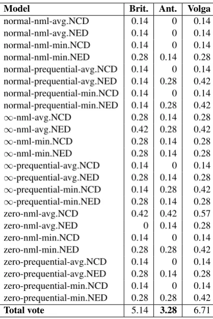
In Table 1, we compare trees generated by the context models to these three gold-standard trees, using the URLL distance defined above.
The context models induce phylogenetic trees as follows. Each model can use prequential coding or NML. Each model yields one NCD matrix and one NED matrix. Finally, for any pair of languages L1 andL2, the model in general produces differ-ent distances for(L1, L2)vs.(L2, L1), depending on which language is the source and which is the target (since some languages preserve more infor-mation than others). Therefore, each of the three context models produces 8 trees, 24 in total. The distance from each tree to the three gold-standard phylogenies is in Table 1.
The measures show which gold-standard tree is
favored by all models taken together. The mod-els strongly prefer “Anttila”—which happens to be the phylogeny favored by a majority of Uralic scholars at present, (Anttila, 1989).
5 Discussion and future work
We have presented an approach to modeling evo-lutionary processes within a language family by coding data from all languages pair-wise. To our knowledge, these models represent the first at-tempt to capture longer-range context in evolu-tionary modeling, where prior work allowed small neighboring context to condition the correspon-dences. We present a feature-based context-aware MDL coding scheme, and compare it against our earlier models, in terms of compression cost and imputation power. Language distances induced by compression cost and by imputation for all pairs of languages, enable us to build complete phyloge-nies. The model takes a set of lexical data as input, and makes no further assumptions. In this regard, it is as objective as possible given the data.11
Finally, we note that our experiments with the context models confirm that the notion of align-ment is secondary in modeling evolution. In the old approach, we aligned symbols jointly, and hoped to find symbol pairs that align to each other frequently. In the new approach, we code sym-bols separately one by one on the source and target level, and A. we code the symbols one feature at a time, and B. while coding each feature, we allow the model to use information from any feature of any symbol that has been coded previously.
These models do better, with no alignment. The objectivity of models given the data opens new possibilities for comparing entire data sets. For example, we can begin to compare the Finnish/Estonian data in StarLing vs. other datasets—and the comparison will be impartial, relying solely on the given data. The models also enable us to quantify the uncertainty of individual entries in the corpus of etymological data. For ex-ample, for a given entryxin languageL1, we can compute the probability thatxwould be imputed by any of the models, trained on all the remaining data fromL1plus any other set of languages in the family. This can be applied in particular to entries marked as dubious by the database creators.
11The data set itself, of course, may be highly subjective.
Acknowledgments
This research was supported in part by the Uralink Project and the FinUgRevita Project of the Academy of Finland, and by the National Cen-tre of Excellence “ALGODAN: Algorithmic Data Analysis” of the Academy of Finland. We thank Teemu Roos for his assistance. We are grateful to the anonymous reviewers for their comments and suggestions.
References
Raimo Anttila. 1989. Historical and comparative linguis-tics. John Benjamins.
Franc¸ois G. Barbanc¸on, Tandy Warnow, Don Ringe, Steven N. Evans, and Luay Nakhleh. 2009. An ex-perimental study comparing linguistic phylogenetic re-construction methods. InProceedings of the Conference on Languages and Genes, UC Santa Barbara. Cambridge University Press.
Alexandre Bouchard-Cˆot´e, Percy Liang, Thomas Griffiths, and Dan Klein. 2007. A probabilistic approach to di-achronic phonology. In Proceedings of the Joint Con-ference on Empirical Methods in Natural Language Pro-cessing and Computational Natural Language Learning (EMNLP-CoNLL:2007), pages 887–896, Prague, Czech Republic.
Alexandre Bouchard-Cˆot´e, Thomas L. Griffiths, and Dan Klein. 2009. Improved reconstruction of protolanguage word forms. In Proceedings of the North American Chapter of the Association for Computational Linguistics (NAACL09).
Rudi Cilibrasi and Paul M.B. Vitanyi. 2005. Clustering by compression. IEEE Transactions on Information Theory, 51(4):1523–1545.
Daniel J. Ford. 2010. Encodings of cladograms and labeled trees. Electronic Journal of Combinatorics, 17:1556– 1558.
Peter Gr¨unwald. 2007. The Minimum Description Length Principle. MIT Press.
David Hall and Dan Klein. 2011. Large-scale cognate recov-ery. InEmpirical Methods in Natural Language Process-ing (EMNLP).
Erkki Itkonen and Ulla-Maija Kulonen. 2000.Suomen Sano-jen Alkuper¨a (The Origin of Finnish Words). Suomalaisen Kirjallisuuden Seura, Helsinki, Finland.
Brett Kessler. 2001.The Significance of Word Lists: Statisti-cal Tests for Investigating HistoriStatisti-cal Connections Between Languages. The University of Chicago Press, Stanford, CA.
Grzegorz Kondrak. 2002. Determining recurrent sound cor-respondences by inducing translation models. In Proceed-ings of COLING 2002:19thInternational Conference on
Computational Linguistics, pages 488–494, Taipei.
Grzegorz Kondrak. 2003. Identifying complex sound corre-spondences in bilingual wordlists. In A. Gelbukh, editor,
Computational Linguistics and Intelligent Text Processing (CICLing-2003), pages 432–443, Mexico City. Springer-Verlag Lecture Notes in Computer Science, No. 2588. Grzegorz Kondrak. 2004. Combining evidence in cognate
identification. In Proceedings of the Seventeenth Cana-dian Conference on Artificial Intelligence (CanaCana-dian AI 2004), pages 44–59, London, Ontario. Lecture Notes in Computer Science 3060, Springer-Verlag.
Petri Kontkanen and Petri Myllym¨aki. 2007. A linear-time algorithm for computing the multinomial stochastic com-plexity.Information Processing Letters, 103(6):227–233. Luay Nakhleh, Don Ringe, and Tandy Warnow. 2005. Per-fect phylogenetic networks: A new methodology for re-constructing the evolutionary history of natural languages.
Language (Journal of the Linguistic Society of America), 81(2):382–420.
Javad Nouri, Jukka Sir´en, Jukka Corander, and Roman Yan-garber. 2016. From alignment of etymological data to phylogenetic inference via population genetics. In Pro-ceedings of CogACLL: the7thWorkshop on Cognitive
as-pects of Computational Language Learning, at ACL-2016, Berlin, Germany, August. Association for Computational Linguistics.
K´aroly R´edei. 1991.Uralisches etymologisches W¨orterbuch. Harrassowitz, Wiesbaden.
Don Ringe, Tandy Warnow, and A. Taylor. 2002. Indo-European and computational cladistics. Transactions of the Philological Society, 100(1):59–129.
Jorma Rissanen. 1996. Fisher information and stochastic complexity. IEEE Transactions on Information Theory, 42(1):40–47.
D.F. Robinson and L.R. Foulds. 1981. Comparison of phy-logenetic trees. Mathematical Biosciences, 53(1–2):131– 147.
Naruya Saitou and Masatoshi Nei. 1987. The Neighbor-Joining method: a new method for reconstructing phylo-genetic trees.Molecular biology and evolution, 4(4):406– 425.
Yuri M. Shtarkov. 1987. Universal sequential coding of single messages. Problems of Information Transmission, 23:3–17.
Sergei A. Starostin. 2005. Tower of Babel: StarLing etymo-logical databases. http://newstar.rinet.ru/.
Hannes Wettig, Suvi Hiltunen, and Roman Yangarber. 2011. MDL-based Models for Alignment of Etymological Data. InProceedings of RANLP: the8thConference on Recent
Advances in Natural Language Processing, Hissar, Bul-garia.