A Method of Transfer Functions and Block Diagrams to Study the Contribution of Variables in Artificial Neural Network Process Models

(1)

Abstract—In this paper is proposed the use of transfer functions and block diagram algebra to describe cause and effect relationships in artificial neural network process models. Explicit formulae are derived for feedforward neural networks with an arbitrary number of inputs, outputs and hidden layers. This novel approach provides a general interpretation of the information existing in neuron interconnections. Numerical applications for the particular case of transfer functions expressed in terms of relative contributions of weights, showed that the method was applicable in the evaluation of the effect of inputs on a given output, with good results.

Index Terms— Variables contribution; Backpropagation; Artificial neural networks; Process modeling.

I. INTRODUCTION

Knowledge of the relative importance of input variables in a neural network model provides two basic advantages [1] - [4]: a) The information can be used to build the optimal neural network model via the selection of inputs, which can improve the generalization capability of the model and allow for faster training of the neural network, with economic savings if measurement of the variables is expensive; b) It provides a better understanding of the process model since the irrelevant variables are identified.

Another point to be considered is that when a great number of input variables are available, but the size of the training set is limited, the likelihood of overfitting is increased [5][6]. In this case, the selection of variables that have the strongest influence on the output is of extreme importance.

Many researchers have tried to express the importance of input variables in neural network models and proposed the use of various methods [3][4][7] -[10].

In the present paper is described a method that uses transfer functions and block diagrams to express input-output dependencies in ANNs, then it is shown that by using this method the concept of analyzing weights to estimate the importance of the inputs can be extended to topological net structures with multiple inputs, multiple outputs and multiple hidden layers.

Manuscript received July 19, 2011; revised August 07, 2011. This work was supported in part by the CAPES and FAPESP.

E.G. Boza-Condorena is the corresponding author.Phone: 19-8119-1822; e-mail: ebozac2003@ yahoo.es.

He is with the School of Chemical Engineering, State University of Campinas, 13083-970, Campinas, SP, Brazil

A.C. da Costa is with the School of Chemical Engineering, State University of Campinas, 13083-970, Campinas, SP, Brazil. (e-mail: [email protected]).

II. THETRANSFERFUNCTIONMETHOD A. Basic concepts

Transfer functions

A transfer function G is a mathematical statement that relates an input, x, to an output, y, of a system [11][12] .

x

y

G



(1) The transfer function G transforms the input x (cause) into an output y (effect)asshown in (2).

y



G

*

x

(2)

Block diagrams

[image:1.595.366.470.437.486.2]

The block diagram can be used to describe cause and effect relationships throughout a dynamic system [13]. Figure 1 shows the block diagram for (2).

Fig. 1. Transfer function

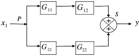
The transfer functions in block diagrams are represented by blocks. The lines that interconnect blocks represent signals that flow interconnecting the system elements. Other components are the pickoff point and the summing point. The four components of a block diagram are shown in Fig. 2. A signal from input x1 flows into the pickoff point (P)

and two signals flow out of the point. In the summing point (S) two signal flows are added, the result is one signal that flows out of the point.

Fig. 2. Blok diagram for transfer functions between input x1 and

output y.

Basic rules of block diagram algebra

The cause and effect relationship between input x1 and output y from the block diagram in Fig. 2 is obtained using

A Method of Transfer Functions and Block

Diagrams to Study the Contribution of Variables

in Artificial Neural Network Process Models

Edwin G. Boza Condorena and Aline Carvalho da Costa

11

G

1

x

21

G

12

G

22

G

y

+

P S

11

G

1

x

21

G

12

G

22

G

y

+

P S

x

G

y

input output

x

G

y

[image:1.595.308.542.622.716.2]

(2)

two basic rules of block diagram algebra, which are: blocks in series combine with each other by multiplication and bocks in parallel combine with each other by algebraic addition. Fig. 3 and Fig. 4 show these two basic rules and the mathematical representation.

Fig. 3. Rule 1: blocks in series

Fig. 4. Rule 2: blocks in parallel

Equation (3) shows the result of applying the basic rules of block diagram algebra first to the blocks in series and then for the resulting blocks in parallel of Fig. 2. Equation (4) is the result of applying the associative property and Equation (5) is the mathematical statement of the transfer function between input x1 and output y. Fig. 5 shows the reduced block diagram obtained from Fig. 2.

1 22 21 1 12

11

*

G

*

x

G

*

G

*

x

G

y





(3)

1 22 21 12

11

*

)

*

(

G

x

y





(4)

)

*

(

11 12 21 22

1 1

G

x

y

_

_

(5)

[image:2.595.79.235.134.386.2]

Fig. 5. Reduced block diagram

Fig. 5 shows that the effect of the input

x

1 on the output

y

is expressed by a transfer function

G

1

.

B. Generalized equations for the effect of inputs on the outputs (EOI)

Notation used

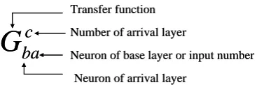
[image:2.595.328.512.137.198.2]

Figure 6 shows the notation used for transfer function in neural networks structure.

Fig. 6. Notation used for transfer function the effect of the input on the output (EOI)

[image:2.595.314.542.319.422.2]

Fig. 7 shows a portion of a neural network structure with one input, two neurons in the hidden layer and one neuron in the output layer. It also presents the transfer function associated to each connection between neurons of adjacent layers.

Fig. 7. Block diagram to show transfer functions in the neural network structure.

From Fig. 7, we obtain the effect of the input on the output (EOI), using the basic rules of block diagram algebra.

2 12 1 21 2 11 1

11

*

G

*

G

[image:2.595.52.264.511.679.2]

E

_OI





(6)

Fig. 8 shows a neural network with two layers and a topology 3: 2: 2.

Fig. 8. Transfer functions in neural network with two inputs, three neurons in the hidden layer and two neurons in the output layer

From Fig. 8, the transfer functions for the effects of each input on the output are the following:

2 13 1 31 2 12 1 21 2 11 1 11

11

G

*

G

*

G

*

G

E





(7)

x

G

₁

y

2

G

x

G

1 +

G

2

y

+ +

x

G

x

G

x

G

y



(

₁



₂

)



₁

*



₂

*

x

G

₁

y

2

G

x

G

1 +

G

2

y

+ +

x

G

x

G

x

G

y



(

₁



₂

)



₁

*



₂

*

x

y

1

G

₂

x

G

x

G

y



₁

*

₂

*



₂

*

₁

*

x

G

1

G

2

y

x

y

1

G

₂

x

y

1

G

₂

x

G

x

G

y



₁

*

₂

*



₂

*

₁

*

x

G

1

G

2

y

x

G

1

G

2

y

y G 1 x 1

G

y

22 21 12

11

*

G

*

G



y

1

x

1

x

y G 1 xGy 1 x 1

G

y

22 21 12

11

*

G

*

G



y

1

x

1

x

Transfer function

Number of arrival layer

Neuron of base layer or input number

Neuron of arrival layer

c

ba

G

Transfer function

c

ba

G

Input Hidden layer (layer 1) Output (layer 2) 1 1 1 2 2 11

G



1 11

G

1 21

G G₁₂2

Input Hidden layer (layer 1) Output (layer 2) Input Hidden layer (layer 1) Output (layer 2) 1 1 1 2 2 11

G



1 11

G

1 21

G G₁₂2

1 1 1 2 2 11

G



1 11

G

1 21

G G₁₂2

[image:2.595.296.543.525.700.2]

(3)

2 13 1 32 2 12 1 22 2 11 1 12

12

G

*

G

*

G

*

G

E





(8)

2 23 1 31 2 22 1 21 2 21 1 11

21

G

*

G

*

G

*

G

E





(9)

2 23 1 32 2 22 1 22 2 21 1 12

22 G *G G *G G *G

E    (10)

From (7) to (10) we can infer that the general equation for effects from input I on the output O, when the feedforward neural network has two layers, with n1 neurons in the hidden layer is,





1

2 1

*

n

j

Oj jI OI

G

E

₍₁₁₎

With a similar procedure were obtained general equations for more complex topologies.

The general equation for effects from input I on the output O, when the feedforward neural network has three layers, with n1 neurons in hidden layer 1 and n2 neurons in layer 2 is:



 



1

1 2

1

3 2 1 n

i n

j

Oj ji iI

OI

G

E

(12)

The general equation for the effect of input I on the output O, when the neural network has r layers, with n(1) neurons in hidden layer 1, n(2) neurons in the hidden layer 2, n (r-1) neurons in the r-1 hidden layer, is:

r r Oi r

r i r i n

i

r n

r i

r n

r i

I i

OI

G

E

1 ₍ ₁₎

) 2 ( ) 1 ( )

1 (

1 ) 1 (

) 2 (

1 ) 2 (

) 1 (

1 ) 1 (

...

_ _ _

 



 

  



(13)

[image:3.595.336.533.159.221.2]

Fig. 9. Algorithm to apply the method of transfer functions

III. NUMERICALAPPLICATIONS

A. Particular case: Relative contributions expressed in

terms of absolute values of the weights as transfer function.

[image:3.595.51.274.422.727.2]

The weights associated to each connection between neurons of adjacent layers were used in transfer functions. Fig. 10 shows the notation used.

Fig. 10. Notation used for weights in neural networks

Equation (14) shows the transfer function expressed as a relative contribution of the absolute values of the weights.





_na

a c ba c ba c

ba

w

G

1

(14)

Where:

G is a transfer function, c is the number of the arrival layer, b is a neuron of the arrival layer, a is a neuron of the base layer or an input number, na is the number of neurons in the base layer or the inputs,

w

_bac is an absolute value of the connection weight,





na

a c ba

w

1

is the sum of the weights that correspond to the connections between the neuron b of the arrival layer and each one of the na neurons of the base layer.

The relative contribution of an input x to an output y, when compared to the relative contributions of the other inputs to the same output, expresses the relative effect of input x on output y, and hence its importance in the set of inputs, as a factor to produce a response y.

Expressing (11) – (13) in terms of relative contributions, we obtain (15) – (17) to estimate the effects of the input variables on the output variables (

E

_OI

)

:

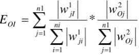
From (11) the general equation in terms of relative contributions as transfer functions for the effects of input I

on the output O, when the feedforward neural network has 2 layers, with n1 neurons in the hidden layer (layer 1), and ni

inputs, is,





 



1

1 2 2

1 1 1

*

n

j

n

j Oj Oj ni

i ji jI OI

w

E

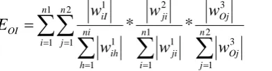
(15)

From (12) the general equation in terms of relative contributions as transfer functions for the effects of input I on the output O, when the feedforward neural network has

Optimize ANN

process model

Define transfer functions

c

ba

G

Estimate the effect of input

I

on the output

O

OI

E

Order of importance of inputs

Optimize ANN

process model

Define transfer functions

c

ba

G

Estimate the effect of input

I

on the output

O

OI

E

Order of importance of inputs

c

ba

w

Weight

c

ba

w

Weight

[image:3.595.308.444.682.736.2]

(4)

3 layers, with n1 neurons in the hidden layer 1,n2 neurons in the hidden layer 2, and ni inputs, can be written:





 



1

1 2

1

2

1 3 3

1

1 1 2

1 1 1

*

n

i n

j

n

j Oj Oj n

i ji ji ni

h ih iI OI

w

E

(16)

Finally, from (13), the general equation in terms of relative contributions as transfer functions for the effect of input I on the output O, when the neural network has r layers, ni inputs, n(1) neurons in layer 1, n(2) neurons in layer 2, … n(r-1) neurons in layer r-1 is:

...

*

...

) 1 (

1 ) 1 (

) 2 (

1 ) 2 (

) 1 (

1 ) 1 (

1 1

) 1 ( 1

) 1 (

  



 



 



n

i

r n

r i

r n

r i

ni

g g i

I i OI

w

E







 

 

   

 

) 1 (

1 ) 1 (

) 1 (

) 1 ( )

2 (

1 ) 2 (

1 ) 2 ( ) 1 ( 1

) 2 ( ) 1 (

*

...

_n_r

r i

r r Oi r

r Oi r

n

r i

r r i r i r

r i r i

w

(17)

Example 1: Neural network with 5: 2: 1 topology, with five inputs, two hidden neurons and one output neuron

[image:4.595.313.537.55.226.2]

In order to test the ability of the proposed method to determine the order of importance of the influence of inputs on outputs, a neural network was trained to describe the process of Isar et al. (2006) [14]. The connection weights of the neural network are shown in Table 1.

Table 1

Example 1: ANN weights associated to each connection between neurons

Hidden layer Output layer

Weights (Wij)

Destination Weights (Wij)

Destination

Neuron 1 Neuron 2 Neuron 1

Source inputs

j =1 j =2 Source O =1

I = 1 4.2452 0.2094 j = 1 0.0436

I = 2 3.2627 0.0638 j = 2 -1.4816

I = 3 14.7474 0.2515

I = 4 9.5223 0.0907

I = 5 0.9688 -0.2702





5

1 1 k

i ji

w

32.7464 0.8856





2

1 2 n

j Oj

w

1.5252

[image:4.595.51.247.79.130.2]

The effects of the inputs on the output,

E

_OI, are obtained using (15) . In this case: ni = 5 (number of inputs), n1= 2 (number of neurons in the hidden layer), O = 1 (number of outputs).

Fig. 2 shows the order of importance of the effects of all the inputs on the output using the transfer function method (Equation 15), the Garson method [7] and the method that uses raw connection weight values [10]. In order to compare the obtained results with the reference values, all the data set was normalized in the range [0.1, 0.9].

0.0 0.1 0.2 0.3 0.4 0.5 0.6 0.7 0.8 0.9 1.0

Input 1 Input 2 Input 3 Input 4 Input 5

Im

p

or

tanc

e

Reference order Tranfer funtion method

Garson method Raw connection weights

Fig. 11. Comparison of the importance of the inputs’ effects using different methods.

The reference order was established using the coefficients of the mathematical model (expressed in terms of coded factors) obtained using experimental design methodology by Isar et al. (2006) [14 ].

In this example, the transfer function method and the Garson method [7] predicted the same order of importance of the inputs as the reference mathematical model [14]. The use of the raw connection weight values proposed by Olden et al. (2004) [10] predicted the order of importance of the inputs erroneously. Two factors that probably contributed to the wrong result were the big difference in magnitude between the highest and the lowest weight values in Table 1 and the great dispersion of weight values around the mean (variance = 23.33). The use of relative contributions expressed in terms of absolute values of connection weights, as transfer functions, as proposed in this work, led to better results in this case.

Example 2: Neural network with 11:5:5:1 topology, to model a batch fermentation process for bioethanol production from sugarcane bagasse

Introduction

The second case study is a process from the work of Andrade et al. (2009) [15]. These authors proposed a mathematical model to describe a batch ethanol fermentation process, and used Plackett-Burman designs [16] to estimate the order of importance of the effects of the kinetic parameters of the mathematical model on the concentrations of biomass (X) and ethanol (P), as well as on the substrate consumption time (t).

[image:4.595.47.293.209.319.2]

(5)

The ‘perturb’ method was applied to build the profiles of the effects of the following inputs on the response: fermentation time for total substrate consumption:

1) µmax = maximum specific growth rate (h -1

)

2) Xmax = biomass concentration when cell growth ceases (kg/ m3)

3) Pm =product concentration when cell growth ceases (kg/ m3)

4)Yx = limit cellular yield (kg/kg)

5)Ypx = yield of product based on cell growth (kg/kg)

6) Ks = substrate saturation parameter (m3/kg)

7) Ki = substrate inhibition coefficient (m3/kg)

8) mp= ethanol production associated with growth (kg/[kg.h])

9) mx = maintenance parameter (kg/[kg.h])

10) m = parameter used to describe cellular inhibition 11) n = parameter used to describe the inhibition by product.

The changes used in the 'perturb' method consisted of variations of -20%, -10%, +10% and +20%, which were produced in the selected input variable around the reference values of the kinetic parameters, while keeping all the other inputs constant. The results are shown in Fig. 13.

7 8 9 10 11 12 13 14 15 16 17 18 19 20 21

-20% -10% 0% 10% 20%

S

ubs

tr

at

e c

o

ns

um

pt

ion t

im

e (

h)

[image:5.595.60.284.312.458.2]

µmax Xmax Pm Ypx Yx Ks Ki mx m n mp

Fig. 12. Profiles of the variation of the output variable according to the changes in the input variables

Fig. 12 shows that there are six inputs with greater influence on the output: Yx, Ypx, _µmax,n, Pm, and Ki.The

most important input affecting the output (fermentation time for total substrate consumption) was Yx, the limit in cell yield (kg/kg).

In order to quantitatively express the information shown in Fig. 13, the S (index) was defined, which measures the cumulative sum of changes in the slope value. The slope is the ratio of the output change to the difference between two consecutive scaled values of inputs, and is calculated by the following equation:



  

 

 ni

i

i i i

i O sI sI O

index S

1

1 1 /

)

( (18)

Where: sI = scaled value of input, O = output value, i = interval number between two consecutive scaled values of inputs.

ANN model topology

With the purpose of applying the transfer functions method, a feedforward neural network with 11:5:5:1

topology, with 11 inputs, 5 neurons in the first hidden layer, 5 neurons in the second hidden layer and 1 output, was selected to model the relationships between the above mentioned factors and the response: fermentation time for total substrate consumption.

The number of neurons in the hidden layers was determined using the cross-validation technique, in order to avoid model overfitting and to achieve good generalization from the training dataset. This technique splits the data sample into a training dataset and a validation dataset. The performance of the trained neural network was evaluated by the ability to predict the elements of the validation dataset, which was expressed in terms of the mean square error (mse).











 N

k

O k k ev t N mse

1

2

1

(19) In (19), k is the number of data points in the validation

dataset, which varies between 1 and N,

t

k is the kth target value, and

ev

O_k is the kth net estimated output value. Comparison of the results for the importance of the effects of input variables on the outputs

The relative importance of all the input variables on a given output using the weight values for this particular ANN structure was obtained using (12).

When the transfer functions are fractional contributions expressed in terms of absolute values of weights,. (12) adopts the form of (16). In this case: ni = 11 (number of inputs); n1 = 5 (number of neurons in the first hidden layer); n2 = 5 (number of neurons in the second hidden layer); O = 1 (output); and I = 1,2,3,…,11 (output number).

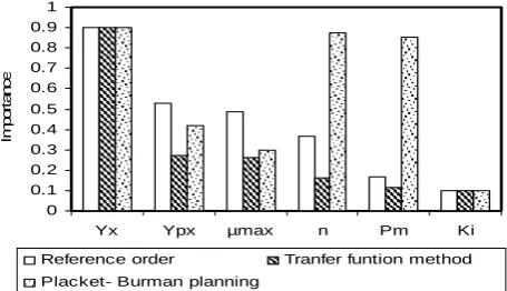
The orders of importance of the six inputs with greater influence on the output, obtained using the transfer function method and the Placket-Burman design [15], are shown in Fig. 13.

0 0.1 0.2 0.3 0.4 0.5 0.6 0.7 0.8 0.9 1

Yx Ypx µmax n Pm Ki

Im

por

tanc

e

Reference order Tranfer funtion method

Placket- Burman planning

Fig. 13 Comparison of the importance of the inputs’ effects on the fermentation time for total substrate consumption, using different methods.

[image:5.595.311.539.506.637.2]

(6)

IV. CONCLUSION

The transfer function method provided a general framework to study the information contained in the weights of ANN based models, which was useful into estimating the importance of inputs on outputs, and facilitated the derivation of applicable equations for models based on neural networks with two or more layers of neurons, extending the possibilities of analyzing these cases with respect to the weight based methods found in the literature.

Transfer functions between adjacent neurons in ANNs could be used to relate inputs and outputs. In numerical applications, good results were obtained when using relative contributions expressed in terms of absolute values of weights as transfer functions, in order to estimate the effects of inputs on outputs.

A good neural network model of a process gives secure information about the relative importance of the input variables, which highlights the importance of the availability of good models to describe the dynamic behavior of chemical and biotechnological processes.

The results showed that the proposed method, which uses transfer functions and the rules of block diagram algebra to estimate the importance of the effects of inputs on outputs in ANN based models, can give better results than the application of Plackett Burman designs.

REFERENCES

[1] A. Engelbrecht, and I. Cloete, “Feature extraction from feedforward neural networks using sensitivity analysis,” In Proceedings of the International Conference on Systems, Signals, Control, Computers, Durban, South Africa,1998, pp. 221-225.

[2] Z. Reitermanová, “Feedforward Neural Networks – Architecture Optimization and Knowledge Extraction,”In WDS'08 Proceedings of Contributed Papers, Part I: Mathematics and Computer Sciences,

Prague, Czech Republic, 2008, pp. 159–164.

[3] Z. Huang, H. Chen, C. J. Hsu, W. H. Chen and S. Wu, “Credit rating analysis with support vector machines and neural networks: a market comparative study,” Decis Support Syst., vol.37, no. 4 , pp. 543–558, Sept. 2004.

[4] J. Tikka, “Simultaneous input variable and basis function selection for RBF networks,” Neurocomputing, vol. 72 no. 10-12, pp. 2649-2658, Jun. 2009.

[5] N. Chapados, and Y. Bengio, “Input decay: Simple and effective soft variable selection,” In Proceedings of the 2001 IEEE/INNS International Joint Conference on Neural Networks, Washington D.C., 2001, pp.1233 – 1237.

[6] T. Similä and J. Tikka, “Combined input variable selection and model complexity control for nonlinear regression,” Pattern Recognit Lett, vol. 30, no. 3, pp. 231-236, Feb. 2009.

[7] G. D. Garson, “Interpreting neural-network connection weights,” AI Expert, vol. 6, no. 7, pp. 47-51, Apr. 1991.

[8] P. Hajela and Z. P. Szewczyk, “Neurocomputing strategies in structural design on analyzing weights of feedforward neural networks,” Struct Multidisc Optim., vol. 8, no. 4, pp. 236-241, Dec. 1994.

[9] Y. Dimopoulos, P. Bourret and S. Lek, “Use of some sensitivity criteria for choosing networks with good generalization ability,”

Neural Process Lett, vol. 2, no. 6, pp. 1-4. 1995.

[10] J. D. Olden, M. K. Joy and R. G. Death, “An accurate comparison of methods for quantifying variable importance in artificial neural networks using simulated data,” Ecol Modell, vol. 178, no. 389-397, Nov. 2004.

[11] W. Luyben, Process modeling, simulation and control for chemical engineers. New York, NY: McGraw-Hill, 1990.

[12] D. E. Seborg, T.F. Edgar, and D.A Mellichamp, Process Dynamics and Control. Hoboken, New Jersey, NJ: John Wiley & Sons, Inc., 2003.

[13] C. Mei, “On Teaching the Simplification of Block Diagrams,” Int J Eng Ed, vol. 18, no. 6, pp. 697-703, My. 2002.

[14] J. Isar, A. Lata, S. Saurabh and S.A. Rajendra, “Statistical method for enhancing the production of succinic acid from Escherichia coli under anaerobicconditions,” Bioresour Technol, vol. 97, pp. 1443–1448, Sept. 2006.

[15] R. R. Andrade, “Procedure for development of a robust mathematical model for alcoholic fermentation process,” M.S. thesis, State University of Campinas, Sao Paulo, Brazil, 2007.