High Performance Computation of Iterative Methods for Matrices Appear in The Field of Realistic Electromagnetics

High Performance Computation of Iterative

Methods for Matrices Appear in The Field of

Realistic Electromagnetics

Takashi Sekimoto

,

Seiji Fujino

Abstract—We estimate performance of the conven-tional and several hybrids of product-type iterative method for solution of realistic electromagnetic prob-lems. Moreover, performance of new coming iteartive methods based on IDR(s) method will be also exam-ined. As a result of total ranking on performance, we will state what iterative method is the most effective through numerical experiments.

Keywords: iterative method, BiCGSafe method, GBi-CGSTAB(s, L) method, electromagnetic problems, pre-conditioning

1

Introduction

We consider to solve efficiently a linear system of equa-tions Ax = b by state-of-the-art iterative methods. Here A means a large, sparse and real nonsymmet-ric coefficient matrix, and x,b is the solution vector and right-hand side vector, respectively. Among many iterative methods, product-type of iterative methods e.g., BiCGStab(Bi-Conjugate Gradient Stabilized)[9] and GPBiCG(Generalized Product-type BiCG)[10] are often used for the purpose of solution for realistic problems. They constitute a sequence of polynomial by multiply-ing Lanczos polynomials by so-called acceleration polyno-mial. The acceleration polynomial is categorized into two groups according to number of term of recurrence That is, BiCGSTAB method is generated by two-term recurrence only, and GPBiCG method is generated by three-term re-currence only. In addition, it must be noted that we meet with instability of GPBiCG method in many numerical experiments.

On the contrary, BiCGSTAB2 [3] method was proposed by M. Gutknecht in 1993. Moreover, same name of BiCGSTAB2 method was proposed as a hybrid version of GPBiCG method by Zhang [10] in 1997. These two types of BiCGSTAB2 methods consist of combinated Lanczos polynomial and acceleration polynomial, and were used for solution of many electromagnetics problems. It is,

∗_{Graduate School of Information Science and Electrical}

Engi-neering, Kyushu University

†_{Research Institute for Information Technology, Kyushu}

Univer-sity Email:[email protected]

however, performance of BiCGSTAB2 methods are de-manded for solution of the large scale problems [11]. Re-cently, on the other hand, various product-type of it-erative methods were proposed one after another, e.g., BiCGSafe [2], GPBiCG AR [4] by the authors and GP-BiCG variant [1] by K. Abeet al. Moreover, a family of IDR(s) [8] such as BiIDR(s) [7] and GBiCGSTAB (s, L) [6] has attracted attention. Therefore, these iterative methods have possibility to supply a demand for gain-ing high performance computgain-ing

In this research, we have two objectives. One of them is that we will implement hybrid methods of BiCGSafe, GPBiCG AR and GPBiCG variant methods as well as BiCGSTAB2 methods. Another of them is that we will evaluate convergence rate of a series of product-type iter-atve method, and a family of IDR(s), and hybrid methods for matrices appear in the field of realistic electromagnet-ics problems.

This paper is organized as follows: In section 2, a brief outline of BiCGsafe2 method as hybrid of the original BiCGSafe method with combination of two-term and three-term recurrences will be described. In section 3, a short description on GBiCGStab(s, L) method includ-ing GBiCG part and MR part will be done. In section 4, computational cost of some iterative methods will be estimated. In section 5, several results of iterative meth-ods will be shown, and it will be made clear that what is the most effective iterative methods through numerical experiments. Finally, in section 6, we have concluding remarks.

2

Hybrid version of BiCGSafe method

We treat with iterative methods for solving a linear sys-tem of equations

Ax = b, (1)

The associate residual a rk is defined as follows:

a rk = rk−ζkArk−ηkyk. (2)

Hererk denotes the residual vector of the algorithm, and y_k denotes also an auxiliary vector. The parametersζk, ηkof the original BiCGSafe method are computed as fol-lows:

ζ = (bk,bk)(ck,ak)−(bk,ak)(ck,bk) (ck,ck)(bk,bk)−(bk,ck)(ck,bk)

, (3)

ηn = (ck,ck)(bk,ak)−(bk,ck)(ck,ak) (ck,ck)(bk,bk)−(bk,ck)(ck,bk)

, (4)

where we impose thatak=rk,bk =yk, ck =Ark.

On the other hand, BiCGSafe2 method with similar prop-erty as BiCGSTAB2 and GPBiCG AR alternates com-putation of parameters ζk, ηk of the original BiCGSafe method. In this approach, we set ηk to be zero at even iteration step. We present an algorithm of BiCGSafe2 method as below.

Algorithm of BiCGSafe2 method

Letx0 be an initial guess,and putr0=b−Ax0

chooser∗0 such that (r0,r0∗)̸=0,setβ−1= 0

fork= 0,1, . . . ,until||rk+1|| ≤ ||r0||do :

begin

pk=rk+βk−1(pk−1−uk−1) (5) Apk=Ark+βk−1(Apk−1−Auk−1) (6)

αk= (rk,r∗0)/(Apk,r∗0) (7)

ak=rk, bk=yk, ck=Ark (8) if mod(k,2)̸= 0, then

ζk= (ck,ak)/(ck,ck), ηk= 0 (9)

uk=ζkApk+βk−1uk−1 (10)

zk=ζkrk−αkuk (11)

yk+1=ζkArk−αkAuk (12) else

ζ= (bk,bk)(ck,ak)−(bk,ak)(ck,bk) (ck,ck)(bk,bk)−(bk,ck)(ck,bk)

(13)

ηn=

(ck,ck)(bk,ak)−(bk,ck)(ck,ak) (ck,ck)(bk,bk)−(bk,ck)(ck,bk)

(14)

uk=ζkApk+ηk(yk+βk−1uk−1) (15)

zk=ζkrk+ηkzk−1−αkuk (16)

yk+1=ζkArk+ηkyk−αkAuk (17) end if

xk+1=xk+αkpk+zk (18)

rk+1=rk−αkApk−yk+1 (19)

βk=

αk

ζk

(rk+1,r∗0)

(rk,r∗0)

(20)

End

3

GBiCGSTAB(

s, L

) method

GBiCGSTAB(s, L) method is derived from GBiCG(s) methods by introducing L-degree stabilization polyno-mial. Computation per iteration of GBiCGSTAB(s, L)

consists of GBiCG(s) part and MR(Minimum Residual) part. In GBiCGSTAB(s, L) method, residual vectorrk, solution vectorxkand auxiliary matrixUk−1are updated

tork+L,xk+L andUk+L−1respectively at everyL

itera-tion. Here,k=mL(m= 1,2, . . .). We denote vectorsrk and matricesUkof GBiCG(s) method asrkGBandUkGB, respectively. Then, we setrk andUk as

rk =Qk(A)rGBk , Uk−1=Qk(A)UkGB, (21) and define approximate solution vectorsxk andxˆ

(i)

k as

b−Axk = rk =Qk(A)rGBk , (22) b−Axˆ(_ki) = rk+i=Qk(A)rGBk+1. (23)

Here, Qk(t) = pm(t)· · ·p2(t)p1(t), product of MR

poly-nomialspi(t)(i= 1,2, . . . , m).

3.1

GBiCG part

In GBiCG part, in k iteration, we update Aj_Q krGBk+L, Aj_QkUGB

k+L₋1, and xˆ (L)

k (j = 0, . . . , L). Here, k = mL(m = 1,2, . . .). First, we give QkrkGB, QkUkGB−1(j =

0, . . . , i), andxk to this part. Next, fori-th iteration(i= 0,2, . . . , L − 1), Aj_Q

kUkGB+i(j = 0, . . . , i) is updated from Aj_QkUGB

k+iet =AjQkrGBk+i−AjQkUkGB+i₋1βk+1(t =

0, . . . , s), and update Aj_Q

krGBk+i+1 from A

j_Q

krGBk+i+1 =

Aj_QkrGB

k+i−Aj+1QkUkGB+iαk+i(j = 0,1, . . . , i). For xˆ

(i)

k , we update such that xˆ(_ki+1) = xˆ_k(i) +αk+iQkUkGB+i Fi-nally this part output Aj_Q

krGBk+L, AjQkUkGB+L₋1, and

ˆ

x(_kL)(j= 0, . . . , L).

3.2

MR part

In MR part, we use output of GBiCG part to up-date residual vector, multiple auxiliary vectors and so-lution vector. First, we choose parameter γ_i(m+1)(i = 1,2, . . . , L) in the L-degree MR polynomial p_m+1(t) = 1−∑L_i=2γ_i(m+1) such that the norm of updating resid-ualrk+L is minimum. Next, from definition ofQk+L(t), Qk+L−1(t) =pt(k)pt(k−L)· · ·p1(t) =pt(k)Qk(t), we up-daterk+L, Uk+Landxk+L as follows:

Qk+LrGBk+L = Qkr

GB

k+L

−

L

∑

i=1

γ(_im+1)AiQkrGB_k+L, (24)

Qk+LUkGB+L−1 = QkU GB

k+L−1

−

L

∑

i=1

γ(_im+1)AiQkU_kGB_+L−1. (25)

From eqns.(23) and (24), xk+L is updated as

xk+L = xˆ

(L)

k −

L

∑

i=1

γ(_im+1)Ai−1QkrGB_k+L. (26)

Algorithm of GBiCGSTAB(s, L) method

Letx0be an initial guess, and putr0=b−Ax0

chooseN×smatricesP0

SetU0= [r0, Ar0, . . . , As−1r0]

SetU1=AU0, M=PTU1,m=PTr0

SolveMγ=mforγ (27)

r0=r0−U1γ,x0=x0+U0γ (28)

r1=Ar0,iter = 0, ω=−1 (29)

While||rn||2/||r0||2> ϵDo

M=−ωM (30)

Fori= 0,1, . . . , L−1 Do

If iter = 0 andi= 0 then i= 1

m=PTri (31)

x0=xiter,r0=riter (32) Forj= 1,2, . . . , sDo

Ifj= 1 then

SolveMγ=mforγ (33)

Ukej=rk− s

∑

q=1

Ukeqγ(q) (k= 0,1, . . . , i) (34)

Else

Solve [m, Me1, . . . , Mej−2, Mej, . . . , Mes]γ =Mej−1 forγ (35)

Ukej=Uk+1ej−1−rkγ(1)− j−2

∑

q=1

Uk+1eqγ(q+ 1)

−

s

∑

q=j

Ukeqγ(q) (k= 0,1, . . . , i) (36)

End If

ComputeUi+1ej=AUiej (37)

Mej=PTUi+1ej (38) End Do

SolveMγ=mforγ (39)

rk=rk−Uk+1γ(k= 0,1, . . . , i) (40)

x0=x0+U0γ (41)

ri+1=Ari (42)

End Do

Forj= 1,2, . . . , LDo

τij= 1

σi

(ri,rj),rj=τijri(i= 1,2, . . . , j−1) (43)

σj= (rj,rj), γ

′

j= 1

σj

(rj,r0) (44)

End Do

γL=γ

′

L, ω=γL (45)

γj=γ

′

j− L

∑

i=j+1

τjiγi(j=L−1, L−2, . . . ,1) (46)

γj′′=γj+1+

L_∑−1

i=j+1

τjiγi+1(j= 1,2, . . . , L−1) (47)

x0=x0+γ1r0,r0=r0−γ ′

LrL, U0=U0−γLUL (48)

U0=U0−γjUj(j= 1,2, . . . , L−1) (49)

x0=x0+γ ′′

jrj,r0=r0−γ ′

jrj(j= 1,2, . . . , L−1) (50) iter = iter + (s+ 1)L (51)

xiter=x0,riter=r0 (52)

End While

4

Estimation of computational cost

Table 1 presents computational cost per one iteration of representative five kinds of methods. In Table 1, “Au” means number of matrix-vector multiplications. “uT_v” means also number of inner products. Similarly “u±v” means number of an addition of two vectors. “αu, u/α” means number of a scalar multiplication of a vector. “N” denotes dimension of matrix, and “N N Z” denotes num-ber of nonzero entries of matrix. Computational cost per (s+ 1) iterations of GBiCGSTAB(s, L) method is shown in Table 1.

5

Numerical experiments

5.1

Computational environment and

condi-tions

All computations were done in double precision floating point arithmetics of Fortran90, and performed on Dell PowerEdge R210 II with CPU of Intel Xeon E3-1220, clock of 3.1GHz, main memory of 8GB and OS of Scien-tific Linux 6.0. Optimum option “-O3” was used. Stop-ping criterion of iterative methods is less than 10−7 of the relative residual 2-norm||rk+1||2/||b−Ax0||2. In all

cases the iteration was started with the initial guess so-lution x0= (0,0, . . . ,0)T. We examined performance of

ierative methods for two matrices which stem from the field of electromagnetic analysis. The iterative methods shown in bold means the hybrid method which combine between two-term and three-term recurrences. In addi-tion, we examined performance based IDR(s) method, i.e., IDR(s), BiIDR(s) and GBiCGSTAB(s, L) methods.

1. GPBiCG, BiCGSTAB,BiCGSTAB2

2. GPBiCG v1, GPBiCG2 v1, GPBiCG v2, GP-BiCG2 v2

3. GPBiCG AR,GPBiCG AR2

4. BiCGSafe,BiCGSafe2

5. IDR(s), BiIDR(s), GBiCGSTAB(s, L)

All test matrices were normalized with diagonal scaling. Maximum iteration was fixed as 10000. ILU(0) precon-ditioning without extra fill-ins are applied to all iterative methods. Acceleration parameter γ for diagonal entries varied from 1.05 until 1.30 at the interval 0.05. The pa-rameter s of IDR(s), BiIDR(s) and GBiCGSTAB(s, L) methods varied as 1, 2, 4 and 8. In a same way, the pa-rameterLof GBiCGSTAB(s, L) method varied as 2 and 3.

Table 1: Computational cost per one iteration of five kinds of methods.

operation GPBiCG BiCGSTAB2 BiCGSafe BiCGSafe2 GBiCGSTAB(s, L)⋆ even odd even odd

Au(×2N N Z) 2 2 2 2 2 2 (s+ 1)

uTv(×2N) 7 7 4 7 7 4 (s2+s+ 3) u±v(×N) 16 16 11 14 14 11 1

2(s

2_L+sL+s2_{+ 5s+L+ 3)}

αu, u/α(×N) 13 13 9 13 13 9 1₂(s2L+sL+s2+ 5s+L+ 3)

Remark: The mark “⋆_{” shows computational cost per (s+ 1) iterations.}

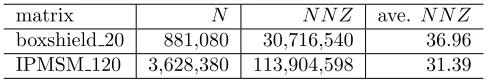
Table 2: Specifications of test matrices.

matrix N N N Z ave. N N Z

boxshield 20 881,080 30,716,540 36.96 IPMSM 120 3,628,380 113,904,598 31.39

by profs. K. Fujiwara and Y. Takahashi of Doshisha University [11]. In Table 2, “N” means number of di-mensions, “N N Z” means number of nonzero entries, and “ave. N N Z” means average number of nonzero entries per one row of matrix.

5.2

Numerical results

Table 3 shows convergence of preconditioned GBiCGSTAB(s, L) method for matrix boxshield 20 when parameter γ is fixed as 1.15. Table 4 presents also convergence of preconditioned GBiCGSTAB(s, L) method for matrix IPMSM 120 when parameter γ is fixed as 1.20. Table 5 exhibits performance of 14 kinds of preconditioned iterative methods for matrix boxshield 20. Similarly, Table 6 shows performance of 14 kinds of preconditioned iterative methods for matrix IPMSM 120. In Table 3-6, “itr.” means number of iterations, and “TRR” means values of True Relative Residual of||b−Axk+1||2/||b−Ax0||2for the converged

solutions xk+1, and “ratio” means ratio of CPU time

of GPBiCG method to that of other iterative methods. From Table 3, as parameterssandLincrease, a number of iterations decreases except for s = 2 for matrix boxshield 20.

Table 3: Convergence of preconditioned GBi-CGSTAB(s, L) method for matrix boxshield 20 when parameterγis fixed as 1.15.

L s itr. total ave. log10

time time (TRR) [sec.] [msec.]

1 1172 116.51 96.49 -7.06 2 2 1188 120.29 98.38 -7.10 4 1070 113.26 102.65 -7.23 8 1062 122.17 111.82 -7.13 1 1146 115.08 97.43 -7.02 3 2 1179 120.84 99.58 -7.17

4 1035 111.49 104.41 -7.04

8 1026 122.75 116.29 -7.03

Table 4: Convergence of preconditioned GBi-CGSTAB(s, L) method for matrix IPMSM 120 when parameterγis fixed as 1.20.

L s itr. total ave. log10

time time (TRR) [sec.] [msec.]

1 1644 674.88 393.49 -7.09 2 2 1218 517.57 401.92 -7.02

4 1060 475.99 422.64 -7.15

8 990 486.63 463.25 -7.08 1 1716 710.82 397.88 -7.08 3 2 1224 527.32 407.87 -7.09 4 1065 487.46 431.36 -7.26 8 999 510.89 483.41 -7.26

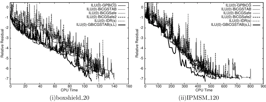
From Table 5, we can gain the following observation.

• GPBiCGSTAB(s, L) method shows the least CPU time, and BiCGSafe method shows the second.

• BiCGSTAB2, BiCGSafe2 and GPBiCG AR2 meth-ods present lower iterations and faster CPU time compared with each original iterative methods.

From Table 6, we get the following observation.

• GPBiCGSTAB(s, L) method shows the least time, and BiIDR(s) method shows the second of that.

• A family of IDR(s) methods present an excellent con-vergence rate.

Table 5: Summary of performance of 14 kinds of preconditioned iterative methods for matrix boxshield 20.

method γ s L itr pre. itr. total ave. log₁₀ ratio ranking time[s] time[s] time[s] time[ms] (TRR)

GPBiCG 1.15 - - 624 3.43 128.08 131.51 205.26 -7.13 1.00 12 BiCGSTAB 1.05 - - 718 3.42 140.94 144.36 196.30 -7.04 1.10 14 BiCGSTAB2 1.10 - - 592 3.43 120.68 124.11 203.85 -7.19 0.94 6 GPBiCG v1 1.10 - - 581 3.43 122.81 126.24 211.38 -7.34 0.96 8 GPBiCG2 v1 1.10 - - 593 3.44 123.38 126.82 208.06 -7.14 0.96 9 GPBiCG v2 1.10 - - 578 3.43 121.35 124.78 209.95 -7.16 0.95 7 GPBiCG2 v2 1.15 - - 612 3.43 127.15 130.59 207.76 -7.15 0.99 11 GPBiCG AR 1.10 - - 579 3.42 118.23 121.65 204.20 -7.20 0.93 4 GPBiCG AR2 1.10 - - 577 3.42 116.94 120.36 202.67 -7.05 0.92 3

BiCGSafe 1.10 - - 582 3.44 119.79 123.23 205.82 -7.27 0.94 5 BiCGSafe2 1.10 - - 575 3.43 116.90 120.33 203.30 -7.07 0.91 2

IDR(s) 1.05 8 - 1010 3.43 134.47 137.90 133.14 -7.05 1.05 13 BiIDR(s) 1.05 4 - 1124 3.44 123.56 126.99 109.93 -7.05 0.97 10 GBiCGSTAB(s, L) 1.15 4 3 1035 3.43 108.06 111.49 104.41 -7.03 0.86 1

Table 6: Summary of performance of 14 kinds of preconditioned iterative methods for matrix IPMSM 120.

method γ s L itr pre. itr. total ave. log₁₀ ratio ranking time[s] time[s] time[s] time[ms] (TRR)

GPBiCG 1.15 - - 859 28.03 719.64 747.67 837.76 -7.13 1.00 12 BiCGSTAB 1.10 - - 1010 28.00 804.74 832.74 796.77 -7.04 1.11 13 BiCGSTAB2 1.20 - - 818 28.04 680.47 708.51 831.87 -7.19 0.95 10 GPBiCG v1 1.15 - - 720 28.02 619.46 647.48 860.36 -7.34 0.87 7 GPBiCG2 v1 1.25 - - 962 28.00 815.82 843.83 848.05 -7.14 1.13 14 GPBiCG v2 1.10 - - 779 27.99 666.82 694.81 855.99 -7.16 0.93 9 GPBiCG2 v2 1.15 - - 823 28.01 696.89 724.90 846.77 -7.15 0.97 11 GPBiCG AR 1.10 - - 683 28.04 571.37 599.40 836.56 -7.20 0.80 5 GPBiCG AR2 1.20 - - 800 28.02 664.54 692.56 830.68 -7.05 0.93 8 BiCGSafe 1.15 - - 654 28.03 543.53 571.56 831.09 -7.27 0.76 4 BiCGSafe2 1.10 - - 744 28.04 616.22 644.26 828.25 -7.07 0.86 6 IDR(s) 1.30 4 - 1042 28.06 541.57 569.64 519.74 -7.05 0.76 3

BiIDR(s) 1.30 4 - 1041 28.02 473.27 501.30 454.63 -7.05 0.67 2

GBiCGSTAB(s, L) 1.20 4 2 1060 27.99 448.00 475.99 422.64 -7.08 0.64 1

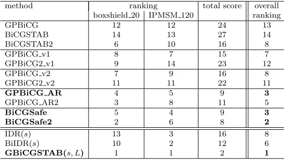
Table 7: Ranking of CPU time and overall for 14 kinds of preconditioned iterative methods.

method ranking total score overall boxshield 20 IPMSM 120 ranking

GPBiCG 12 12 24 13

BiCGSTAB 14 13 27 14

BiCGSTAB2 6 10 16 8

GPBiCG v1 8 7 15 7

GPBiCG2 v1 9 14 23 12

GPBiCG v2 7 9 16 8

GPBiCG2 v2 11 11 22 11

GPBiCG AR 4 5 9 3

GPBiCG AR2 3 8 11 5

BiCGSafe 5 4 9 3

BiCGSafe2 2 6 8 2

IDR(s) 13 3 16 8

BiIDR(s) 10 2 12 6

-7 -6 -5 -4 -3 -2 -1 0

0 20 40 60 80 100 120 140 160

Relative Residual

CPU Time

ILU(0)-GPBiCG ILU(0)-BiCGSTAB ILU(0)-BiCGSafe ILU(0)-BiCGSafe2 ILU(0)-IDR(s) ILU(0)-GBiCGSTAB(s,L)

-7 -6 -5 -4 -3 -2 -1 0

0 100 200 300 400 500 600 700 800 900

Relative Residual

CPU Time

ILU(0)-GPBiCG ILU(0)-BiCGSTAB ILU(0)-BiCGSafe ILU(0)-BiCGSafe2 ILU(0)-IDR(s) ILU(0)-GBiCGSTAB(s,L)

(i)boxshield 20 (ii)IPMSM 120

Figure 1: History of relative residual 2-norm six kinds of methods.

6

Concluding Remarks

In this paper, we examined convergence rate of sev-eral product-type iterative methods and a family of and IDR(s) based on iterative methods for two matri-ces stemed from FEM analysis for electromagnetic prob-lems. Through numerical experiment, it turned out that GBiCGSTAB(s, L)andBiCGSafe2methods have ef-fectiveness and robustness compared with the other iter-ative methods. We will analyse effect of SSOR precondi-tioning with Eisenstat trick. We would like to consider mathematical theory and aspect as a future work.

Acknowledgments

We show sincere thanks to profs. K. Fujiwara and Y. Takahashi of Doshisha University for giving interesting two matrices stemed from FEM analysis for realistic problems. We appreciate an anonymous referee for giving nice advise (see ref.[1]).

References

[1] K. Abe, G.L.G. Sleijpen, Solving linear equations with a STABilized GPBiCG method, Proc. of 14th Kansetouchi workshop of JSIAM, pp.29-34, Okayama University of Science, January, 2011.(in print)

[2] S. Fujino, M. Fujiwara and M. Yoshida, BiCGSafe method based on minimization of associate residual, JSCES No.20050028, 2008.

[3] M. H. Gutknecht, Variants of BiCGStab for matri-ces with complex spectrum, SIAM J. CSI. Comput, Vol.14, pp.1020-1033, 1993.

[4] Moethuthu, S. Fujino, Stability of GPBiCG AR method based on minimization of associate residual, Journal of ASCM, Vol.5081, pp.108-120, 2008.

[5] Moethuthu, S. Fujino, A variant of GPBiCG AR method with reduction of computational costs, Asian Technology Conference in Mathematics (ATCM), pp.419-428, Thailands, December, 2008.

[6] M. Tanio, M. Sugihara, GBi-CGSTAB(s, L): IDR(s) with higher-order stabilization polynomials, J. of Computational and Applied Mathematics, Vol.235, pp.765-784, 2010.

[7] M.B. van Gijzen, P. Sonne veld, An elegant IDR(s) variant that efficiently exploits bi-orthogonality properties, TR 08-21, Delft Univ. of Tech., 2008.

[8] P. Sonneveld, M.B. van Gijzen, IDR(s): a family of simple and fast algorithms for solving large non-symmetric linear systems, SIAM Journal on Scien-tific Computing, Vol.31, pp.1035-1062, 2008.

[9] H. A. van der Vorst. Bi-CGSTAB: A fast and smoothly converging variant of Bi-CG for the solu-tion of nonsymmetric linear systems, SIAM J. Sci. Stat. Comput., pp.631-644, 1992.

[10] S.-L. Zhang, GPBi-CG: Generalized product-type preconditionings based on Bi-CG for solving non-symmetric linear systems, SIAM J. Sci. Comput., pp.537-551, 1997.