Generic Sensor Model Development and Simulation of Degradation Effects

3954

©IJRASET: All Rights are Reserved

Generic Sensor Model Development and Simulation

of Degradation Effects

Sreeraj S

Software Engineer, Continental Automotive Components Pvt Ltd, India

Abstract: Sensors play a crucial role in the functioning of Autonomous cars. All ADAS and Autonomous driving (AD) functions especially those associated with high safety levels, require rigorous test drive of millions of kilometres for the qualification. This much amount of real test drive is not practically possible with any car manufacturer. So, there is a high demand for a test strategy where the function will be validated in virtual test drive environment. This can reduce the necessary efforts for the qualification of a given function and its validation. To realize virtual testing, the closed loop of the environment, vehicle and the driver should be modelled for simulation. The interface between the environment and the vehicle which converts the physical information into electrical signals is the sensor. The sensor is highly important in ADAS and AD function as it replaces the role of a driver in the car. So, for virtual testing it is required to model a generic sensor which can simulate the complete behaviour of any real sensor which is used in the vehicle. This paper focuses on the modelling of major degradations applied on the ground truth data due to the sensor. So here the input to the sensor model will be the traffic objects data which are dimensions of each traffic object and output will be the traffic object list with degraded dimensions.

Keywords: ADAS (Advanced Driver Assistance System), AD (Autonomous Driving), Sensor model, Traffic Object, FOV (Field of View), Simulation

I. INTRODUCTION

Reliable AD (Autonomous Driving) and ADAS (Advanced Driver Assistance System) functions are of crucial importance these days as many of these functions are mandatory as per the statutory regulatory bodies in USA and Europe. Since many performance qualification requirements directed by the government must be fulfilled and the complexity of the vehicle is also constantly increasing, the validation of AD and ADAS functions is getting more expensive and time consuming [1]. This is the situation where automotive component suppliers are forced to deliver behaviour sensor models to the vehicle manufacturers. Late failure detections usually lead to a lot of corrections in the software and additional maintenance time and cost. Compromising on the quality and functional safety for AD and ADAS function is not at all acceptable. Therefore, the concern is how to achieve maximum test coverage and thus to ensure the reliability on a product or a driver assistance feature.

Going for test drives which is conventional way is not a practically feasible method for validation. As per the directives from safety regulatory bodies, a test drive of 50 Lakh kilometre is required to certify that a particular function is roadworthy [5]. Also, for autonomous vehicle, various fatal accidents are also reported during the real road test drives. Simulation is promising method to test and validate any AD and ADAS function due to the following benefits

A. Critical safety situations can be tested in virtual setup B. Various environments can be involved in the test C. Testing activity can be made faster than real time

D. Man hours can be drastically reduced which will reduce the cost

Also, modelling and validating radar and camera sensors is of high importance today as most of the ADAS features like Lane Departure warning, Adaptive Cruise Control, Warnings based on traffic signs take input from these sensors. In this paper, the model architecture and the concepts behind the different behaviours of the sensors is detailed. A generic sensor is modelled in Simulink. The test environment or the complete test scenario is created in Carmaker.

3955

©IJRASET: All Rights are Reserved

II. MODEL ARCHITECTURE

The sensor model mainly consists of two sections as shown in Fig. 1. First section is the input s-functions blocks which gets Carmaker data [4]and also the sensor configuration which is set from an external Graphical User Interface. A GUI is developed in Visual Studio for selecting sensors and its parameters. Also, there is a visual studio project for Carmaker [4]. The Carmaker data and the sensor data is passed to windows shared memory. This is to share data between two processes i.e. Matlab and Visual Studio. So, the S-functions in the Matlab which is programmed in C++ can access the data in windows shared memory using corresponding APIs [2]. The ground truth data from Carmaker and sensor parameters is fed to the Sensor Logic block. The main task of this block is to filter the ground truth information by either passing, removing or manipulating data inside the object list. The specific factors which affect the sensor behaviour are Field of view which defined by range distance, range of horizontal and vertical angle, distance of a target object from sensor, sensor mounting position, focal length and pixel resolution in case of camera sensors etc. Sensor behaviour affects the visibility or detectability of an object by the sensor. Fig. 2 illustrates the general working of the Sensor model. For example, properties of n number of ground truth objects are given as input to the sensor model. The model modifies the object list based on the visibility of object. This modification of the object properties. due to sensor behaviour is called object degradation. The ground truth and detected object list is an m×n matrix where m is the number of properties of the object and n is the number of objects. In this model each traffic object is assumed as a cuboidal box (Fig. 3) and the following properties of the object is used (relative to ego-vehicle):

1) Object centre position in x direction (longitude) in metre. 2) Object centre position in y direction (latitude) in metre.

3) Object centre position in z direction (from ground) in metre. 4) Object velocity in x direction in metre per second.

5) Object velocity in y direction in metre per second. 6) Length, width and height of the object.

Fig. 1. Overview of Sensor Model architecture Fig. 2. Input and Output structure of Sensor Model

Sensor Logic block contains functional blocks connected in a sequence. Each functional block corresponds to different behaviours of the sensor. The major behaviours or the degradation effects modelled in the Sensor Logic block is as follows

a) Latency b) FOV filtering

c) FOV and Object occlusion d) False Negative and Positive

e) Imager resolution (Only for camera sensors) f) Measurement Error

Concept behind each behaviour listed above is briefed in the next section.

3956

©IJRASET: All Rights are Reserved

III.SENSOR BEHAVIOUR CONCEPTS

A. Latency

Electronic components present in the sensor circuit can contribute to a delay of few microseconds between the input and output of the sensor. Suppose a car is detected at t=10 sec. But the sensor will output car information only after a few microseconds. This is called Detection latency. The sensor configuration GUI has the provision to configure the latency time. Model will take the latency time as an input. During simulation, latency in detection is represented as change in position along x and y coordinates of the traffic object. The object position due to latency is calculated as follows:

X = X + (Vel_X * Latency_time) Y = Y + (Vel_Y * Latency_time)

In the above equations X is the longitudinal position and Y is the latitude position of the position. Vel_X and Vel_Y are the vehicle velocities in longitudinal and latitude direction respectively. Latency_time is the latency time in microseconds range converted in seconds. Due to latency, the longitude and latitude positions of the object is shifted by a distance which is equivalent to the velocity in the corresponding direction multiplied by the latency time.

This is how latency effect is realized in each simulation step.

B. FOV filtering

Based on the sensor parameters like range, horizontal and vertical angular ranges, the model calculates the Field of View region. The objects which are completed out of FOV will be discarded or eliminated from further processing. For this, all the eight corner points of the object is calculated and if at least one corner is inside the FOV, the object will be considered for further processing otherwise it will be discarded.

C. FOV Occlusion and Object Occlusion

When the sensor cannot detect some portion of object or the complete object due to either object is partially inside FOV or due to one object hiding another.

If some of object corner points are inside the FOV and the rest are outside, the object is partially occluded by FOV. In this case the portion of the object which is outside of FOV is truncated by reducing the object dimensions and portion which is inside is retained. This shows the sensor behaviour that it can detect only the portion of object which is in its field of view. This is FOV occlusion. The second type of occlusion is Object occlusion where an object will be completely inside the FOV, but it will be partially or completely hidden by another object. Object occlusion algorithm is briefed below:

1) Calculate the distance of each object from sensor

2) Calculate azimuth and elevation angle of all corner points of each object 3) Calculate the extreme azimuth and elevation angle of each object 4) Sort the object in ascending order of distance from sensor

5) If the azimuth sector of the second object is outside that of first object, retain the second object else if azimuth sector of the second object is completely inside that of first object, check if elevation sector of second object is completely inside that of first object. If yes, remove the second object else reform the object size and retain the object.

D. False Negative and False Positive

False negative situation happens when some objects which are actually present in the field of view will not be detected as an object. This happens when the radar or camera sensor fails to recognize an object. This happens in a random fashion.

This random behaviour is modelled in the following way: 1) Find the total number of objects till the 20th _{simulation cycle.}

2) Number of false negative objects will be calculated for every 21st _cycle.

3) Number of false negative objects will be the total number of objects in last 20 cycles multiplied by the false negative factor. False negative factor is a user input to the model.

4) Then from the object list some number of objects equivalent to number of false negative objects will be removed randomly at the 21st _{cycle. False positive detection means sensor provides information about objects which are not actually present in FOV.}

This detection decision is caused by noise or other interfering signals exceeding the detection threshold. Probability of False positive objects are more near to FOV boundary due to influence of noise.

3957

©IJRASET: All Rights are Reserved

6) Number of false positive objects will be calculated for every 21st _cycle.

7) Number of false positive objects will be the total number of objects in last 20 cycles multiplied by the false positive factor. False positive factor is a user input to the model.

8) Then from the object list some number of objects equivalent to number of false positive objects will be added randomly at the 21st _cycle.

E. Imager resolution (Camera Sensors)

Object degradation is inversely proportional to the imager resolution i.e. lesser the resolution, more the object degradation. Minimum number of pixels required for object detection is user configurable in sensor configuration GUI. Object degradation algorithm is as follows.

For a given camera focal length and FOV, imager width and height are calculated using following relation

where

1) hfov=horizontal field of view (in degrees) 2) vfov= vertical field of view (in degrees) 3) F=focal length in (mm)

4) v= vertical dimension of sensor (height of imager) (mm) 5) h= horizontal dimension of sensor (width of imager) (mm) Using the above two equations, find the height and width of imager. a) Pixel resolution is calculated as below:

i) Pixel width resolution= v/pixel dimension in width ii) Pixel height resolution= h/pixel dimension in height

b) Calculate Objects length, width, height in image plane using following relation i) Wc = (Wa * f)/d ---(1)

ii) Hc = (Ha * f)/d ---(2) iii) Lc = (La * f)/d ---(3)

Where

d = distance of object center w.r.t camera position (m). f = focal length of camera (mm).

Wc, Hc, Lc = object width, length, and height in image co-ordinate system (mm).

Wa, Ha, La =object real width, length and height respectively in vehicle co-ordinate system(m).

Object width in image is calculated using equation (1). Then calculate the random error between zero and pixel width resolution. Introduce twice the calculated random error on object image width to consider the degradation effect on both sides of object width. Use the relation shown in equation (1) to get object’s real width with resolution error.

To find the image resolution effect on object height, above steps have to repeated with random error chosen between 0 and pixel height resolution. Use the relation shown in equation (2) to get object’s real height with resolution error. Pixel length resolution is the average of pixel height resolution and pixel width resolution. So, in the same way image resolution effect on object length to be calculated with random error chosen between 0 and pixel length resolution. Use the relation shown in equation (3) to get object’s real length with resolution error.

F. Measurement Error

Radar measurements are subjected to random errors when the rising edge of the echo signal is distorted by noise. In real radars measurement error can happen in the calculation of object centre position and dimensions. In this sensor model , the measurement error is modelled in the following way:

3958

©IJRASET: All Rights are Reserved

L, W - length, width respectively.

L’, W’ - L, W after addition of measurement error respectively. X, Y -Object center .

X’, Y’ - X, Y Object center after addition of measurement respectively. n - Measurement error with Gaussian noise associated.

IV.FUNCTIONAL TESTING AND RESULTS

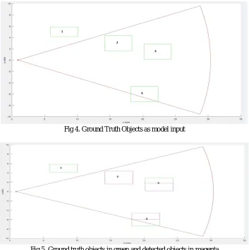
Model is simulated with four traffic objects as input. The objects are positioned as shown in Fig. 4 which is plotted in Matlab. The sensor input is configured with a range of 30 m. FOV can also be seen in the same figure. In Fig. 4, Object 1 is placed out of FOV . Object 2 is clearly visible to the sensor. Object 3 is placed behind the Object 2 so Object 3 is only partially visible to the sensor. Object 4 is partially out of FOV.

Fig. 5 shows both the ground truth and detected objects. Ground truth objects are shown in green colour. Detected objects are shown in magenta colour.

Fig 4. Ground Truth Objects as model input

Fig 5. Ground truth objects in green and detected objects in magenta

Object 1 is not detected at all as it is completely out of FOV. Object 2 is completely detected. Object 3 is partially detected as it is partially occluded by Object 2. Object 4 is also partially detected as it is partially out of FOV. Results are as expected.

V. CONCLUSIONS

3959

©IJRASET: All Rights are Reserved

REFERENCES

[1] Hanke, T., Hirsenkorn, N., Dehlink, B., Rauch, A., Rasshofer, R., Biebl, E. (2015): Generic architecture for simulation of adas sensors. In 2015 16th international radar symposium, IRS (pp. 125–130). https://doi.org/10.1109/IRS.2015.7226306.

[2] Hanke, T., Hirsenkorn, N., van Driesten, C., Garcia-Ramos, P., Schiementz, M., Schneider, S. K. (2017): Open simulation interface—a generic interface for the environment perception of automated driving functions in virtual scenarios.

[3] Hirsenkorn, N., Hanke, T., Rauch, A., Dehlink, B., Rasshofer, R., Biebl, E.(2016): Virtual sensor models for real-time applications. Adv. Radio Sci., 14,31– 37. https://doi.org/10.5194/ars-14-31-2016. U R L : https://www.adv-radio-sci.net/14/31/2016/.

[4] IPG Automotive GmbH: CarMaker

[5] Krajzewicz, D., Erdmann, J., Behrisch, M., Bieker, L. (2012): Recent development and applications of SUMO—simulation of urban Mobility. Int. J. Adv. Syst. Measur.,5(3&4), 128–138.