Development of trip generation equations for the Gold Coast and Sunshine Coast regions

Full text

(1)Bachelor Thesis. Development of Trip Generation Equations for the Gold Coast and Sunshine Coast Regions. Veitch Lister Consulting Brisbane, Australia. 08 February 2008. Robert van Beilen s0043753.

(2) Trip Generation. Veitch Lister Consulting. Trip Generation Review and development of the VLC Trip Generation Equations for the Gold Coast and Sunshine coast region. Veitch Lister Consulting P/L, Suite 3, Ground Floor, 80 Jephson Street, Toowong, QLD 4066, Australia. http://www.veitchlister.com.au Daily supervisor: Tim Veitch. Twente University Faculty of Engineering Technology Civil Engineering (& Management) Drienerlolaan 5 7522 NB Enschede http://www.cit.utwente.nl Supervisors: prof. dr.ir. E. (Eric) C. van Berkum dr. T.(Tom) Thomas. Author: R. (Robert) J. van Beilen Waalstraat 219 7523 RG Enschede r.j.vanbeilen@student.utwente.nl. Van Beilen. 2. 2/8/2008.

(3) Trip Generation. Veitch Lister Consulting. Executive Summary The current method of modelling trip production in Veitch Lister Consulting’s Trip Generation Model is to use simple linear regression with stratified household attributes included as dummy 0-1 variables. While this is effective for calculating average trip rates for various household attributes, the nature of the data is such that the assumptions of linear regression are seriously violated. This means that the usefulness of these averages applied at various levels is questionable and measures of model accuracy are not to be trusted entirely. A technique commonly cited in the literature for accommodating the assumptions of linear regression with count data is to take a log transform of those counts. However, in this case, the data is also heavy in zeros and so a log transform will actually worsen the performance. In fact there is no transformation that can ‘spread out’ a large number of zeros to make data suitable for simple linear regression. Instead, Zero-Inflated Poisson and ZeroInflated Negative Binomial models are proposed as an improvement and assume to be more effective in modelling count data heavy in zeros. These zero-inflated models however, are non-linear and thus it is not possible to simply apply them at the equations zonal (aggregate) level as can be done with linear models. This report details the model assumptions, fit, diagnostics and performance for each of the six trip production purposes under the linear regression technique. The zero-inflated models are finally discussed as possible future improvements but this will need some further investigation and research.. Van Beilen. 3. 2/8/2008.

(4) Trip Generation. Veitch Lister Consulting. Table of Contents Executive Summary................................................................................................................................. 3 1. Introduction....................................................................................................................................... 7. 2. Personal Objectives ......................................................................................................................... 8. 3. Research Plan.................................................................................................................................. 9 3.1. Company profile................................................................................................................. 9. 3.2. Project & Research Description....................................................................................... 10. 3.2.1. Background...................................................................................................................... 10. 3.2.2. Problem analysis ............................................................................................................. 10. 3.2.3. Objectives ........................................................................................................................ 11. 3.3 3.3.1 3.4. 4. Research Questions ........................................................................................................ 13 Central questions ............................................................................................................. 13. 3.4.2. Sub questions .................................................................................................................. 13. Dataset Description ........................................................................................................................ 14 Data Preparation.............................................................................................................. 15. 4.1.1. Definition of Population.................................................................................................... 15. 4.1.2. Definition of a Trip............................................................................................................ 15. 4.1.3. Table production .............................................................................................................. 16. 4.2. Characteristics of the home interview sample – household structure ............................. 17. 4.3. Summary.......................................................................................................................... 22. Trip Generation Literature Review ................................................................................................. 23 5.1. Introduction ...................................................................................................................... 23. 5.2. Zones and networks ........................................................................................................ 24. 5.2.1. Background...................................................................................................................... 24. 5.2.2. VLC’s SEQ Transport model ........................................................................................... 24. 5.3. Classification.................................................................................................................... 25. 5.3.1. Trip purpose..................................................................................................................... 25. 5.3.2. By Time of Day ................................................................................................................ 26. 5.3.3. By Person Type ............................................................................................................... 26. 5.4. 6. The research model ......................................................................................................... 12. 3.4.1. 4.1. 5. Methodology .................................................................................................................... 11. Factors affecting Trip Generation .................................................................................... 27. 5.4.1. Factors affecting production ............................................................................................ 27. 5.4.2. Factors affecting attraction .............................................................................................. 27. 5.5. Category analysis ............................................................................................................ 28. 5.6. Regression analysis......................................................................................................... 29. Methodology................................................................................................................................... 32 6.1. Van Beilen. Calibration........................................................................................................................ 32. 4. 2/8/2008.

(5) Trip Generation. 6.2 7. Veitch Lister Consulting. Validation ......................................................................................................................... 33. Comparison of models ................................................................................................................... 34 7.1 7.1.1. Formulation and fit ........................................................................................................... 35. 7.1.2. Performance .................................................................................................................... 35. 7.2. nd. 2 Regression model ...................................................................................................... 37. 7.2.1. Formulation and fit ........................................................................................................... 38. 7.2.2. Performance .................................................................................................................... 38. 7.3 8. st. 1 Regression model ....................................................................................................... 34. Cross Classification ......................................................................................................... 40. Results ........................................................................................................................................... 42 8.1. Calibration........................................................................................................................ 42. 8.2. Validation ......................................................................................................................... 43. 9. 8.2.1. Home based trip productions........................................................................................... 43. 8.2.2. Cross classification trip rates ........................................................................................... 44. Discussion ...................................................................................................................................... 46 9.1. Log-linear model .............................................................................................................. 46. 9.2. Zero-inflated models ........................................................................................................ 47. 10. Conclusion and Recommendations ................................................................................. 49. 11. References....................................................................................................................... 51. Appendix 1. Household Travel Survey Summary............................................................................ 54. 1.1. Why was the Survey Needed?........................................................................................... 54. 1.2. What are the Survey Objectives? ...................................................................................... 54. 1.3. What was the scope of the Survey? .................................................................................. 54. 1.4. Definition of Terms............................................................................................................. 54. 1.5. Time period and Methodology ........................................................................................... 55. 1.6. Target population ............................................................................................................... 56. 1.7. Sample size and composition ............................................................................................ 57. 1.8. Interpretation of the results ................................................................................................ 57. 1.9. Summary............................................................................................................................ 58. Appendix 2 2.1. Dummy variable regression......................................................................................... 59 VLC’s stratified dummy variable regression ...................................................................... 59. Appendix 3. Assumptions and descriptions..................................................................................... 61. 3.1. Multicollinearity .................................................................................................................. 61. 3.2. Linear regression ............................................................................................................... 61. 3.3. Correlation matrix............................................................................................................... 62. Appendix 4. VLC model coefficients................................................................................................ 63. Appendix 5. Model output................................................................................................................ 64 st. 5.1. 1 Regression model run ................................................................................................... 64. 5.2. 2 Regression model run (stepwise)................................................................................. 71. Appendix 6. Van Beilen. nd. Diagnostics .................................................................................................................. 87. 5. 2/8/2008.

(6) Trip Generation. Veitch Lister Consulting. Table of Figures figure 1: The south east Queensland region ......................................................................................... 10 figure 2: Nested relationship of trip purposes........................................................................................ 14 figure 3: Broad structure of SEQ Households ....................................................................................... 18 figure 4: Histograms of the number of households by person categories and cars .............................. 20 figure 5: Histograms of number of trips of all trip purposes................................................................... 21 figure 6: Traditional 4-step Model .......................................................................................................... 23 figure 7: VLC SEQ zoning ..................................................................................................................... 24 figure 8: Ordinary least squares regression .......................................................................................... 29 figure 9: Illustration of stratified dummy linear regression with and without intercept.. ......................... 32 figure 10: Log-linear histograms of transformed trip rates of HBW_White and HBS ............................ 46. table 1: Reclassification of trip purposes............................................................................................... 16 table 2: Example HH_structure.............................................................................................................. 16 table 3: Example Home Based Trip count per HHID per Purpose Category ........................................ 16 table 4: Example stratified dummy variable table.................................................................................. 17 table 5: Broad structure of SEQ_HHTS................................................................................................. 17 table 6: Structure of SEQ_HHTS – Workers – Dependants – Cars ...................................................... 19 table 7: Common predictors in trip production models .......................................................................... 24 table 8: Overall trip purposes as in the SEQ household survey data.................................................... 25 table 9: VLC’s Trip purpose categories ................................................................................................. 25 table 10: SEQ Occupation descriptions specified to VLC definitions .................................................... 26 table 11: Cross-classification by workers and dependants ................................................................... 28 table 12: trip production model coefficients, calibration results home-based person trips per HH (1). 34 table 13: Comparison of estimated against observed home based person trip productions (1)........... 36 table 14: trip production model coefficients, calibration results home-based person trips per HH (2).. 37 table 15: Comparison of estimated against observed home based person trip productions (2)........... 39 table 16: summary of trip rates by household structure(1).................................................................... 40 table 17: summary of trip rates by household structure(2).................................................................... 41 table 18: Summary of calibration results ............................................................................................... 42 table 19: mean absolute- and weighted trip production error per trip purpose ..................................... 44 table 20: mean absolute- and weighted trip rate error per classification category................................ 45 table 21: Percentage of zeros for each trip purpose in the whole dataset ............................................ 47 table 22: SEQTS summary.................................................................................................................... 58 table 23: Correlation matrix ................................................................................................................... 62 table 24: VLC Trip Generation Coefficients........................................................................................... 63. Van Beilen. 6. 2/8/2008.

(7) Trip Generation. Veitch Lister Consulting. 1 Introduction The purpose of this report is to analyse the effectiveness of the current method of modelling trip generation used in Veitch Lister Consulting’s (VLC) transport model and to propose alternatives. It provides an independent review of the trip generation equations as described in the technical report, Calibration of an Integrated Travel Forecasting model [VLCTN2, 1997]. The data used in the existing VLC model was collected from 1992/1995, incorporating data from 5565 households from Melbourne. The model was then tested against the 1992/’94 Household Travel Survey Data for the Brisbane Statistical Division and is currently implemented in the South East Queensland region. To facilitate an analysis the model structure will be recalibrated using available 2004/’05 South East Queensland Household Travel Survey (SEQHTS) data to obtain updated parameters and model fit estimates. The current method of predicting trip productions is to use ordinary linear regression with dummy variables, see Ortuzar, J. de D. and Willumsen (1994) for an introduction. Briefly trips are split by purpose and for each purpose a separate regression equation is calculated relating the number of trips (for each purpose) to household attributes (such as the number of workers, dependants or vehicles). It is a relatively simple method of allowing zonal totals to be used as inputs for the model equations. However, some of these models have a very low explanatory power and violate some basic statistical assumptions of linear regression. These assumptions are that the range of dependant variables is unrestricted, the dependant and independent variables are linearly related, and that errors are normally distributed, uncorrelated with constant variance (that is, homoskedastic). The dummy formulation is used to avoid issues of non-linear relationships, but does not address the problems created by the restricted range of the dependent variable (i.e. the number of trips con only be positive) nor the non-normal, heteroskedastic errors. The use of simple regression is further complicated by the presence of a large number of zero trips for all trip purposes. Thus the main objection to the current models is that the distribution of the variables is not appropriately considered. Often trip generation models use a log transform to account for the restricted range of the dependent variable and the heteroskedastic errors. However, the literature says count data with values close to zero may be more effectively modelled in a generalised linear model (GLM) framework with a Poisson distribution. The traditional alternative to linear regression is category analysis or cross-classification. This tends to have higher data demands than regression techniques, and does not provide measures of model fit or accuracy. As a result, the following components are successively described in this report: • First of al an outline of my personal objectives –what I want to accomplish– are presented; • This is followed by an outline of the research plan which actually form the guiding principles how to tackle the problem; • Chapter 4 gives an overview of the data collection and necessary preparations executed for this research; • The literature on both regression and category analysis are reviewed in the following part; • Chapter 6 outlines the specific methodology that has been used for updating the model; • In chapter 7 the results of each model are given and compared in chapter 8; • This is followed by a discussion and notion of possible future improvements; • Finally conclusions and recommendations are given in the last chapter.. Van Beilen. 7. 2/8/2008.

(8) Trip Generation. Veitch Lister Consulting. 2 Personal Objectives Before starting with the description of the research a short outline of my personal objectives (i.e. what I personally want to learn/accomplish with this project) is presented. These objectives will mainly concern knowledge and experience that I would like to gain in the field of traffic and transport engineering. 1) To get a better understanding of the actual field of work I would first of all like to learn and get more familiar with the use of transport related theories (e.g. trip generation, trip distribution, modal split and assignment etc.) in real-life projects. Questions I am asking myself regarding this case are: What part of the theory is really coming back in practice? What information/data is necessary to write a good and reliable traffic model? 2) I want tot gain knowledge about the use of OmniTRANS and the Zenith (VLC’s transport modelling software) in practice as a tool for travel demand forecasting, transportation- / land use planning and traffic engineering. 3) Third thing I want to gain experience in is the consultancy work. The models are used to predict and simulate traffic, but what is actually done with the outcome? What does a typical advice look like? To what extend is the consultancy involved in the progress of a project? Hopefully this internship will answers my questions and gives more insight the practical work of a consultancy in the field of transportation planning and traffic forecasting.. Van Beilen. 8. 2/8/2008.

(9) Trip Generation. Veitch Lister Consulting. 3 Research Plan 3.1. Company profile. Veitch Lister Consulting Pty Ltd (VLC) is one of the largest specialist transport and traffic planning consultancies in Australia. Established in 1986 by Mike Veitch, VLC specializes in providing a full range of transport planning services including: • • • • • • • • • • • • •. Travel demand forecasting (including model development and associated software); Transportation planning and policy development; Toll road revenue and demand forecasting; Public transport policy, route strategy and service planning; Traffic micro-simulation; Traffic engineering, parking analysis and local area traffic management; Socio-economic analysis; Economic evaluation; Studies of land use/transport interaction; Survey design, data collection, statistical and market analysis; Bicycle path and trail planning; Special event planning; and Transport planning training.. The company combines the skills of some of Australia’s best transport planners and traffic engineers to offer a wide range of services to the public and private sectors. VLC has built on the extensive expertise of its staff to successfully complete assignments throughout Australia and in South-East Asia. The company offers particular expertise in the areas of travel demand forecasting, toll modelling and public transport modelling and planning. VLC has revolutionized transport modelling in Australia, with the development of highly accurate travel forecasting models, which support planners in developing the most pragmatic and efficient solutions to a wide range of transport problems. VLC has invested 20 years, and millions of dollars in developing its models, which are by far the most accurate, sophisticated and well-researched in Australia. In particular their public transport models are at the cutting edge of world research, and are designed specifically for Australian conditions. The modelling techniques developed by VLC have become industry standard within Australia. With Australia’s most powerful modelling tools at their disposal, VLC’s transport planning staff are able to add significant value in all areas of transport planning. Importantly, many of VLC commissions make use of their own integrated transport modelling software, ZENITH. This comprehensive modelling software allows detailed time-period modelling of both private and public transport. Integrated models can be used to estimate car and truck flows as well as a wide range of public transport data including trip patterns, boardings and alightings and load profiles. The ZENITH model starts from a detailed description of the land uses within the modelled area to develop transit and vehicle trip patterns from ‘first principles’. The assignment of these trip tables to the modelled infrastructure network is also state-of-the-art. Presentation of results is first class through integration with a graphical information system (GIS). VLC’s experience and technical expertise are highly regarded within the industry. VLC has been involved in the planning and modelling of several hundred major projects over an extended period of time, with a focus on close client collaboration, and providing the client with pragmatic, innovative and useful solutions [VLC Company Profile, 2007].. Van Beilen. 9. 2/8/2008.

(10) Trip Generation. 3.2. Veitch Lister Consulting. Project & Research Description. 3.2.1 Background 1 Veitch Lister Consulting is the developer (and owner) of a comprehensive four-step model of the South-East Queensland (SEQ) region. SEQ is a rapidly growing region of the state of Queensland and actually is the fastest growing region in Australia, fuelled principally by migration from the southern states. The SEQ region contains approximately two-thirds of the state population and is estimated to be 2.8 million which is heavily urbanised and concentrated along the coast. The three largest population areas are concentrated in Brisbane, Gold Coast and the Sunshine Coast which subsequently account for 90 per cent of the region's population. Future development plans of South East Queensland focus on slowing down coastal development, in order to prevent creating a 200 km city, and instead aim for growth in the west [WIKIQLD, 2007], [SEQIPP, 2007]. The modelled area spans nearly 400 km north-to-south, and nearly 200 km east-to-west, and is frequently utilized on a wide variety of transport planning and modelling projects. The Transport authorities and Planning agencies are required to make decisions on transport infrastructure and services worth billions of dollars. The decision making process for transport planning needs to be informed, accountable and founded on comprehensive, current and reliable figure 1: The South-East Queensland Region data. One of the most important areas of information needed is an accurate description of travel behaviour of the people living in this area. The most effective way for transport planners to gather this information is by the conduct of a household travel survey. The last time a survey of this nature was conducted in South-East Queensland was in 1992/’94. This data is now dated and hence it was decided to conduct a new travel survey. The purpose of this research project is to re-calibrate the trip generation component of the model in light of newly available household travel survey data.. 3.2.2 Problem analysis The existing trip generation equations of the SEQ model are not up to date and based on 1992/’95 Melbourne survey data. The model was then tested against the 1992/’94 Household Travel Survey Data for the Brisbane Statistical Division. There are demographical differences between the South East Queensland region and the cities of Brisbane and Melbourne. The SEQ region consists of retired people and tourists highly. Furthermore it is clear that the SEQ region is undergoing fast changes in terms of growth. Currently the model under predicts traffic and the existing equations are manipulated manually to compensate for these drawbacks. So if VLC wants to say something credible about future developments in the region it would be highly implausible if their arguments and predictions are based on the 1992/’95 Melbourne and Brisbane data they currently use for their models. But what drives people to move to this region and what is the purpose of their trips? The newly available household 1. The four step model is formed by: 1) Trip Generation – how many trips, of what purpose 2) Trip Distribution – where people travel to? By using the gravity model 3) Modal Split – the different modes of transport 4) Assignment. Van Beilen. 10. 2/8/2008.

(11) Trip Generation. Veitch Lister Consulting. travel survey data should give a better prediction of the factors that influence trip generation in the region.. 3.2.3 Objectives As mentioned before, the overall objectives of this project for VLC are to have an updated version of the existing model in light of the newly available household travel survey data. The importance of this research lies in the fact that VLC wants to be able to give founded and justified recommendations, with the updated model, concerning future developments. With this advanced investment, VLC is able to be ahead of competition when new transport infrastructure projects are being planned. Having this model up to date gives the organisation the opportunity to state plausible travel demand forecasts and get involved in future development plans in early stages. The objectives of my research are: 1. To gain a full understanding of the scope, structure and reliability of the new household travel survey, for the purposes of developing a four-step travel model 2. To gain a full understanding of VLC’s current trip generation techniques, and to gain “handson” experience in using these techniques on a real-life project 3. To evaluate the soundness of VLC’s trip generation techniques in comparison to other techniques; both theoretically, and empirically. 4. To implement a re-calibrated trip generation model for use in future VLC projects. Summarizing; the objective of my thesis is to develop a new trip generation model for the South East Queensland region by giving insight in the newly available household travel survey data and by analysing the existing trip generation model in the light of other trip generation techniques which will give VLC the opportunity to be ahead of competition and state more plausible travel demand forecasts for the region.. 3.3. Methodology. The execution of the project can be broken down into a number of stages that are described in the following sub-sections. Familiarisation First of all I will start with the ‘familiarisation’ stage. This will involve: Investigation of the household travel survey – an extensive report including all the household travel survey data and an explanation/procedure manual of the survey is available. A working paper listing relevant questions of interest has been prepared (see research questions section paragraph 3.4). Following investigation of these questions, a short summary document should be produced describing and summarising the key features of the survey. Introductory reading relating to trip generation – Chapter 4 of the text “Transport Modelling” by Ortuzar et al. should be read as introductory reading to trip generation. Introduction to VLC’s current trip generation techniques – a technical note describing the original calibration of VLC’s trip generation model will be provided, and should be read. Following this, a VLC staff member will provide a hands-on demonstration of the currently implemented trip generation model. Finally, I will prepare a short report summarising VLC’s currently implemented techniques. Development of a New Trip Generation Model When the familiarisation stage is finished the imposed development of the new trip generation model can start. This stage will involve:. Van Beilen. 11. 2/8/2008.

(12) Trip Generation. Veitch Lister Consulting. Selection of a statistics package – a statistics technique (e.g. regression analysis or variance analysis) will need to be chosen to sort the data and remove inaccuracies. This can be done with R-project, SPSS, SAS or another statistics package. Data Preparation - The household travel survey data will need to be cleaned, and manipulated into a form that is suitable for input into the statistics package. Re-calibration of VLC’s existing trip generation equations – As a starting point, it will be useful to recalibrate the trip generation equations that VLC currently uses. The validation of this new model should then be compared with the validation of the “old” equations using the survey data. Finally, the new equations should be implemented in VLC’s model, to investigate how they affect overall model performance against traffic counts. Calibration of other model forms – following a review of the literature, some attention should be devoted to other forms of trip generation models. Their performance should be compared to the recalibrated versions of VLC’s trip generation equations, with a judgement made about which should be adopted. Implementation and Presentation The initial plan was to implement the proposed new trip generation model within VLC’s standard model, and consider its implications for overall model calibration. Due to time constraints, as well personal as within the organisation this did not occur. 3.3.1 The research model To make sure the objectives of my research are going to be achieved it is useful to make a clear overview of the different stages that have to be accomplished to reach the final goal. The research model below is a schematic reproduction of the project and the global stages that are going to be executed. Investigation of the household travel survey data. Summarising report about SEQ HTS and Trip Generation recommendation.. Reviewing the literature regarding Trip Generation. Gain hands-on VLC’s existing trip generation techniques. Investigation of Statistical Techniques. Develop a Trip Generation model for the South-East Queensland region. 1) VLC’s existing trip generation equations. 2) SEQ region. (a). (b). (c). (a) Investigation of the household travel survey, reviewing the available literature relating to trip generation modelling and getting hands on the existing trip generation techniques should lead to a report containing new insights and recommendations for improvement of the existing model (b). In this report, the factors/parameters that influence trip generation in the SEQ region are presented by which the performance of VLC’s existing trip generation techniques can be evaluated. (c) This will finally lead to the development of a new trip generation model for the South-East Queensland region and implementation within VLC’s standard model.. Van Beilen. 12. 2/8/2008.

(13) Trip Generation. 3.4. Veitch Lister Consulting. Research Questions. It is clear that my research aims on a practical application with the objective of re-calibrating VLC’s existing trip generation equations. The objective asks for prescriptive knowledge that should give a proposal on how the model should be updated. To be able to do this, more knowledge concerning the background of the existing model and the purpose of the project is necessary. This will mainly be explanatory information that comes across by making inquiries. For that reason, the research is split up in central- and sub questions to get better insight.. 3.4.1 Central questions The answers to the central questions should tend to be sufficient to accomplish the overall objective of my research and are formulated as follows: 1. Why is a new trip generation model for the South East Queensland region necessary? 2. What criteria does the survey data need to satisfy to be reliable and useful for trip generation modelling? 3. What factors influence trip generation in the South East Queensland region? 4. To what extent does the existing VLC model meet the required outcomes? 5. To what extent do other trip generation models meet the required outcomes?. 3.4.2 Sub questions The sub questions are mainly meant to support and answer the central questions. The following sub questions are formulated: 1.1. 1.2.. What is VLC’s purpose with the new trip generation model? On what data is the existing trip generation model of the SEQ region based?. 2.1. 2.2.. 2.6.. What purposes of travel are reported? How many trips of each type are there? How is the time of the trip recorded? How precise? Is it the start or end of the journey, or are both recorded? How are the origin and destination of the trip recorded? District? Suburb? Address? Or perhaps coordinates? What household attributes are recorded? Number of people? Number of cars? Etc. What individual attributes are recorded? Occupation (Employed/Student/Unemployed) – what categories? What categories of employment? What dates are the surveys conducted? Beginning/End, during school holidays?. 3.1. 3.2.. What factors affecting trip generation appear from the Household Travel Survey Data? What other factors, that did not appear from the survey, should be taken into account?. 4.1. 4.2.. What factors affecting trip generation are currently taken into account for the existing model? To what extent an update of the existing model is necessary?. 5.1.. What factors affecting trip generation are taken into account in other trip generation models following a review of the literature? How do other trip generation models perform regarding to trip predictions?. 2.3. 2.4. 2.5.. 5.2.. Van Beilen. 13. 2/8/2008.

(14) Trip Generation. Veitch Lister Consulting. 4 Dataset Description This chapter starts with a short description how the survey data has been collected and which trip purposes are accounted for in this research. This is the actual basis and first part of my research and describes the household travel survey data and its overall characteristics. Paragraph 4.1 outlines the necessary data preparation that has been made for the development of the trip generation equations. For a full description of the household travel survey data I would like to refer to Appendix 1. The Household Travel Survey collected data in the form of travel diaries from approximately 7000 households. Each household filled in the diary for a representative working day, during October – November 2003 or February – March 2004. Holidays have been avoided as good as possible but some private school and university holidays were unavoidably included. The previous 1992 Household Travel Survey had drawn a random sample from residential Energex (Energy Company) billing addresses and used a mail out – mail back survey. This sampling methodology was changed slightly for the 2003/’04 SEQTS to improve a dropping response rate observed in other cities. It was decided to change to a hand delivery – hand collection system, with follow-up telephone calls to encourage the completion of questionnaires. To facilitate this more labour intensive method a two-step process was used when sampling. First, census collection districts (CCD’s) were sampled (320 out of 4185), and then households were randomly sampled within each district (at the rate of approximately 6%). Using these techniques the target response rate of 60% was maintained for the Brisbane region (60%) and the Sunshine Coast (62%). The response rate for the Gold Coast reached a reasonable (55%). The variables pertinent to this research are: the number of trips (by purpose); household structure (blue collar, white collar and undefined workers, dependants by age groups A[0-17], B[18-64], C[65+] and household vehicles. (See following pages for full variable descriptions and histograms of responses). The nested relationship of the trip purpose is shown in figure 2.. Home Based Work. Home Based Education. White Collar. Primary/ Preschool. Blue Collar. Undefined. Tertiary. Secondary. Non Home Based. Home Based Other. Work based Other Work based Shopping. Recreation. Work based Work. Shopping. Shopping based Shopping. Other. Shopping based Other. Other Non Home Based. figure 2: Nested relationship of trip purposes. The blue shaded groups are taken into account while the non-home based travel is not considered in this analysis.. Van Beilen. 14. 2/8/2008.

(15) Trip Generation. 4.1. Veitch Lister Consulting. Data Preparation. The data as collected during the survey period and provided in the database can not be used directly for the development of the trip generation equations. The data namely is incomplete or missing in some cases, collected during school holidays, inconsistent or incorrectly classified. Furthermore data is also collected from visitors who normally aren’t residents of the area. All these data needs to be filtered and excluded from the survey since they affect the trip generation calculations in a negative way which of course needs to be avoided.. 4.1.1 Definition of Population The entire survey contains a total population of 18.194 people. Visitors are included in the TotalPersons per household variable of the data, though they are not counted as household members and so not included in the HHsize variable. So HHsize is the variable we are interested in for household size (i.e. not including visitors). PersonIDs from people who are not residents (i.e. RESIDENT = 2) are filtered out, which leaves 17.783 PersonIDs remaining. As mentioned in table 22, Appendix 1, total number of responding households is 6.978. While preparing the data it became clear that some records were inconsistent in terms that the count of PersonIDs in the household (where RESIDENT = 1) did not match the HHsize. In other words, where the number of people recorded did not match the household size. This situation (after removing the visitors) covers 10 household cases. These households have been removed from the data since it is impossible to discover what the actual values should be. In total these 10 households matched 34 people, which have been removed and left 6.968 HHIDs and 17.749 PersonIDs remaining. Further investigation brought another inconsistency to the light. Some people seemed to note Home_Based_Work(HBW) trips without specifying their occupation. Effect on the trip generation in this case is that it is impossible to specify the trip as a Blue or White collar worker trip. Households that recorded unspecified HBW trips in this case where also entirely ignored and excluded from the data. In total 668 trips in 216 households were of this type of unspecified HBW trips, 216 HHIDs and all matching PersonIDs (i.e. 274) have been removed, remaining 6.752 HHID and 17.475 PersonIDs. Households who were interviewed during school holidays / tertiary holidays actually need to be filtered out. From the 2003 and 2004 school calendar it became clear that the survey never was executed during public primary and secondary school holidays. But private school holidays and tertiary holidays tend to differ in some way from the public school holidays. This has actually not been taking into account since this would only be a small portion and it is hardly impossible to find out all private school holidays. So the final sample size contains 6752 households.. 4.1.2 Definition of a Trip The Access database of the survey contains a “SEQTS_TRIPS” table in which each individual person trip is recorded. If a trip involves interchanging then each “leg” will be recorded in the “SEQTS_STOPS” table, but the trip will only be recorded once in the trips table. So, the definition of a trip used for trip generation is a row in the trips table. For each trip a “Start Purpose”, “End Purpose” and “Overall Purpose” are recorded. After the first regression though, it looked like the classification as specified in the survey was not done properly or at least not as expected by VLC. The main problem noticed after regression in comparison with the existing VLC model, arose in a big difference between observed and estimated “Home Based Education”(HBE), “Home Based Other”(HBO) and “Home Based Recreation” (HBR)-trips. From this we could read that the total number of observed HBE_PrePrim(Pre- & Primary school)-trips were 2,65 times the model estimated. For HBE_Sec(Secondary) the observed trips were twice as much as estimated. And for the HBR applies they were underpredicted by a factor 1,6. On the other hand HBOtrips though were highly over predicted (almost 4 times as many as observed). This seeming shift from trips to different purposes was a reason to have a closer look at the different classifications of the Home Based-trips whereas especially accompanying and serving passenger trips where differently specified than expected. table 1 shows these trips and their specified overall purpose as given in the survey. The last column in the table shows the desired VLC purpose, which in each case is HBO for these specific trips. Reason for the proposed changes lies in the fact that even though someone’s trip might have the specified destination (e.g. education, shopping, social or work) doesn’t mean their. Van Beilen. 15. 2/8/2008.

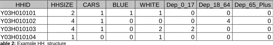
(16) Trip Generation. Veitch Lister Consulting. individual trip purpose is of the specified classification. All incorrectly specified trips are changed and recoded into the desired VLC overall purpose. Start Purpose Home Home Accompany EducationPrim Serve Pass. EducationPrim. End Purpose Accompany EducationPrim Serve Pass. EducationPrim Home Home. Overall Purpose HBE - Pre Primary HBE - Pre Primary HBE - Pre Primary HBE - Pre Primary. VLC Overall Purpose Home Based Other Home Based Other Home Based Other Home Based Other. Home Home Accompany EducationSec Serve Pass. EducationSec. Accompany EducationSec Serve Pass. EducationSec Home Home. HBE - Secondary HBE - Secondary HBE - Secondary HBE - Secondary. Home Based Other Home Based Other Home Based Other Home Based Other. Home Home Accompany EducationTert Serve Pass. EducationTert. Accompany EducationTert Serve Pass. EducationTert Home Home. HBE - Tertiary HBE - Tertiary HBE - Tertiary HBE - Tertiary. Home Based Other Home Based Other Home Based Other Home Based Other. Home Home Serve Pass. Pers. Bus/Welfare Serve Pass. Shopping. Serve Pass. Pers. Bus/Welfare Serve Pass. Shopping Home Home. Home Based Shopping Home Based Shopping Home Based Shopping Home Based Shopping. Home Based Other Home Based Other Home Based Other Home Based Other. Home Serve Pass. Social/Ent/Recreation. Serve Pass. Social/Ent/Recreation Home. Home Bases Social Home Bases Social. Home Based Other Home Based Other. Home Based Work Home Based Work. Home Based Other Home Based Other. Home Serve Pass. Work Related Bus. Serve Pass. Work Related Bus. Home table 1: Reclassification of trip purposes. 4.1.3 Table production The structure of VLC’s trip production model is a series of additive linear relationships (one for each trip purpose) that describe the number of person trips made by households of varying characteristics on a typical weekday where there are seven stratified attribute groups (SAG’s) that in itself are a linear function as well. How these so called “dummy variables” exactly work is explained Appendix 2. First step in gaining the desired data is producing a table from the Access database that describes the household structure of each of the remaining 6.752 households in terms of the specified attribute groups. table 2 is an example of the produced table. HHID Y03H010101 Y03H010102 Y03H010103 Y03H010104. HHSIZE 2 4 4 1. CARS. BLUE 1 1 1 0. WHITE Dep_0_17 Dep_18_64 Dep_65_Plus 1 0 0 0 0 0 4 0 2 2 0 0 1 0 0 0. 1 0 0 0. table 2: Example HH_structure. This table tells us something about the household size (HHSIZE), #cars (CARS), #blue collar workers (BLUE), #white collar workers, dependants aged 0-17 (Dep0_17), dependants aged 18-64 (Dep18_64) and dependants aged 65+ (Dep_65_plus), per household. Next step is to get information about the observed trip counts per households, per purpose. table 3 tells something about the total number of home based trips that have been produced by each household. Home based trips can be split up in eight different purposes – i.e. Education Pre/Primary, Education Secondary, Education Tertiary, Other, Shopping, Recreational, Blue Collar and White Collar trips. HHID Y03H010101 Y03H010102 Y03H010103 Y03H010104. HBE_PP HBE_SEC HBE_TER 0 0 0 0 0 4 0 3 0 0 0 0. HBO 0 0 0 0. HBS 8 5 4 0. HBR HBW_BL HBW_WH 2 2 0 1 0 0 1 0 2 0 0 2. table 3: Example Home Based Trip count per HHID per Purpose Category. Van Beilen. 16. 2/8/2008.

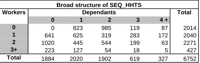
(17) Trip Generation. Veitch Lister Consulting. From the tables above, a table of all households with a field for each stratified dummy variable and the number of trips, looking like table 4 below, is produced for each trip purpose. This set of 14 excel sheets containing 6752 rows (one for each household) and 32 columns (HHID, one for each dummy variable and trip count) are created by use of programming language “’Ruby”. HHID. HHSIZE_1. Y03H010101. HHSIZE_2 0. BLUE_0. HHSIZE_3 1. BLUE_1 0. WHITE_0. BLUE_2 1. WHITE_1 0. Dep0_17_0. Dep0_17_1. 1 1 CARS_0. HBE_PP_Trips 0. 0 Dep0_17_3. 0 Dep18_64_2. Dep0_17_4+ 0. 0. Dep18_64_3+ 0. 0. Dep_65+_2+ 0. CARS_1. 0. 0. 0. 0 Dep_65+_1. HHSIZE_6+ 0. WHITE_3+. Dep0_17_2. Dep18_64_0 Dep18_64_1 Dep_65+_0. 0. 0. HHSIZE_5 0. BLUE_3+. WHITE_2 1. 1. HHSIZE_4 0. 0 CARS_2. 0 1 table 4: Example stratified dummy variable table. CARS_3+ 0. 0. From the examples above we can read that household Y03H010101 has a household size of two, containing one blue collar worker, one white collar worker, zero dependants, one car and doesn’t make any HBE_PP_Trips. This sounds quite logical since this household does not have any dependant household members in the age group of 0 – 17 who will basically make trips to pre- and primary school. Now we have the household structure and the observed number of trips per purpose of each household in the survey.. 4.2. Characteristics of the home interview sample – household structure. The broad structure of the South East Queensland household sample is presented in table 5 with respect to the worker and the dependants attribute of households. Workers are considered as the sum of white collar and blue collar workers (see paragraph 5.3.1 for an explanation of different worker types). Dependants are presented as the sum of the co-occupying household members in the age groups of 0-17, 18-64 and 65+. For example, there are 319 households with 1 worker and 2 dependant co-occupiers in the entire survey. A more comprehensive breakdown of the household structure of the sample is presented in table 6, where the data construct adopted for table 5 is layered bye household car ownership.. Workers 0 1 2 3+ Total. 0 0 641 1020 223 1884. Broad structure of SEQ_HHTS Dependants 1 2 3 823 985 119 625 319 283 445 544 199 127 54 18 2020 1902 619. Total 4+ 87 172 63 5 327. 2014 2040 2271 427 6752. table 5: Broad structure of SEQ_HHTS. Van Beilen. 17. 2/8/2008.

(18) Trip Generation. Veitch Lister Consulting. Furthermore the following histograms in figure 3 provide a better understanding of the household structure in the SEQ travel survey data. 2.500. 2.500. 3.000. Mean =1,35 Std. Dev. =1,175 N =6.752. Mean =1,18 Std. Dev. =0,968 N =6.752. 2.000. Mean =2,53 Std. Dev. =1,301 N =6.752. 2.500. 2.000. 1.000. Frequency. Frequency. Frequency. 2.000. 1.500. 1.500. 1.500. 1.000 1.000. 500. 500 500. 0. 0 0. 1. 2. 3. 4. 5. 6. 7. 8. 9. 10. Total_Dependants. 0. 0. 1. 2. 3. Total Workers. 4. 5. 6. 0. 1. 2. 3. 4. 5. 6. 7. 8. 9. Hhsize. figure 3: Broad structure of SEQ Households. An appreciation of the structure of the household sample is important when considering the adequacy of the model in replicating the behaviour of various market segments. Interesting points to note from table 5, table 6 and the corresponding figures are: Referring to table 5 and figure 3 it can be seen that the average household size in the survey approximately is 2,53 persons per household, which sounds realistic and doesn’t impose a closer look. The most common household contains two workers and no dependants followed closely by households containing no workers and two dependants instead (15,1 over 14,6 percent). Furthermore it is interesting to note there are about an equal number of zero worker-, one worker- and two worker households (28,9 percent, 30,2 percent and 33,6 percent respectively). The fact there are that much zero worker households sounds somewhat conspicuous so a closer look to this group tells there are: - 280 zero worker households with dependants in the category 65+, zero cars - 842 zero worker households with dependants in the category 65+, one car - 213 zero worker households with dependants in the category 65+, two cars - 23 zero worker households with dependants in the category 65+, three+ cars This means that of all 2014 zero worker households, a total of 1358 are actually households with merely retirees which is 67,4 percent respectively. The more comprehensive breakdown of the household structure, layered by car ownership, is presented in the following table 6:. Van Beilen. 18. 2/8/2008. 10. 11. 12.

(19) Trip Generation. Veitch Lister Consulting. Structure of SEQ_HHTS – Workers – Dependants - Cars car ownership = 0 Workers Dependants Total 0 1 2 3 4+ 0 0 278 85 15 6 384 1 66 25 11 2 3 107 2 10 4 2 1 0 17 3+ 2 0 0 0 0 2 Total 78 307 98 18 9 510 car ownership = 1 Workers 0 499 235 16. Dependants 1 2 506 624 284 136 69 72 7 2. 63 70 18 0. 49 36 7 0. 750. 866. 834. 151. 92. 0 66 686 54. 31 277 251 32. Dependants 1 2 254 136 364 15. 36 178 133 3. 26 108 33 0. 806. 591. 769. 350. 167. 8 39 121 88 256. Dependants 1 2 22 36 106 37 201. 0 0 1 2 3+ Total. car ownership = 2 Workers 0 0 1 2 3+ Total. car ownership = 3+ Workers 0 0 0 1 10 2 89 3+ 151 Total 250. Total 3. 4+ 1242 1025 401 25 2693. Total 3. 4+. 3 5 33 47 15 100. 4+ 6 25 23 5 59. 347 765 1467 104 2683. Total 41 143 386 296 866. table 6: Structure of SEQ_HHTS – Workers – Dependants – Cars. From the table above it is interesting to note that only 510 out of 6752 households (7,6 percent) do not have access to a motor vehicle and the number of households with access to three motor vehicles or more even exceeds the number of non-car owning households. Furthermore the number of two car owning households can almost be said to be equal to the number of one car owning households. Further information about the household structure can be found in figure 4 where histograms and frequency tables of the number of dependants, blue- and white collar workers and number of cars are presented. Information about total trips per purpose is presented in the histograms of figure 5.. Van Beilen. 19. 2/8/2008.

(20) Trip Generation. Veitch Lister Consulting. 5.000. 6.000. 5.000 Mean =0,44 Std. Dev. =0,669 N =6.752. Mean =0,58 Std. Dev. =0,982 N =6.752 4.000. Mean =0,33 Std. Dev. =0,63 N =6.752. 5.000. 4.000. 2.000. Frequency. Frequency. Frequency. 4.000 3.000. 3.000. 3.000. 2.000 2.000. 1.000. 1.000. 0. 1.000. 0. 0 0. 1. 2. 3. 4. 5. 6. 7. 8. 0. 1. 2. Dep_0_17. 4. 1. Percent. Frequency (HH). 4631. 68,6. 1. 818. 12,1. 1. 1860. 2. 903. 13,4. 2. 3. 451. 315. 4,7. 4. 3. 70. 1,0. 62. 5. 13. ,2. 6. 1. 7. 1. ,0. 6752. 100,0. Dep_65_Plus 0. 64,8. Frequency (HH). Percent 76,1. 27,5. 1022. 15,1. 6,7. 2. 589. 8,7. ,9. 3. 3. ,0. 7. ,1. Total. 6752. 100,0. 6752. 100,0. 3.000. Mean =0,35 Std. Dev. =0,591 N =6.752. Mean =0,83 Std. Dev. =0,847 N =6.752. 2.500. 4. 1. 5.000. 3.000. 3. 5138. 4. ,0. Percent. 4372. Total. 2. Dep_65_Plus. Dep_18_64 0. Total. 0. 5. Dep_18_64. Frequency (HH). Dep_0_17 0. 3. Mean =1,62 Std. Dev. =0,915 N =6.752. 2.500. 4.000. 1.500. Frequency. 2.000. Frequency. Frequency. 2.000. 3.000. 1.500. 2.000 1.000. 1.000. 1.000 500. 500. 0. 0 0. 1. 2. 3. 4. 5. 6. 0. 0. 1. White_CW. White_CW 0. 2. 3. 4. 5. 6. 0. 1. Blue_CW. Frequency (HH). Percent. Blue_CW 0. 2. 3. 4. 5. 6. 7. 8. Cars. Frequency (HH). Percent. Frequency (HH). Cars. Percent. 2878. 42,6. 4756. 70,4. 0. 510. 7,6. 1. 2327. 34,5. 1. 1664. 24,6. 1. 2693. 39,9. 2. 1389. 20,6. 2. 303. 4,5. 2. 2683. 39,7. 3. 133. 2,0. 3. 24. ,4. 3. 628. 9,3. 4. ,1. 4. 186. 2,8. 1. ,0. 5. 48. ,7. 100,0. 6. 2. ,0. 7. 2. ,0. 6752. 100,0. 4. 23. ,3. 4. 5. 2. ,0. 5. Total. 6752. 100,0. Total. 6752. Total figure 4: Histograms of the number of households by person categories and cars Van Beilen. 20. 2/8/2008.

(21) Trip Generation. Veitch Lister Consulting. 6.000. 4.000 Mean =0,46 Std. Dev. =0,973 N =6.752. 5.000. Mean =0,94 Std. Dev. =1,317 N =6.752 3.000. Frequency. Frequency. 4.000. 3.000. 2.000. 2.000 1.000 1.000. 0. 0 0. 1. 2. 3. 4. 5. 6. 7. 8. 9. 10. 0. 1. 2. 3. HBW-Blue_Trips. 4. 5. 6. 7. 8. 9. 10. HBW-White_Trips. 6.000. 7.000 Mean =0,36 Std. Dev. =1,015 N =6.752. 5.000. 7.000 Mean =0,23 Std. Dev. =0,763 N =6.752. 6.000. Mean =0,07 Std. Dev. =0,416 N =6.752. 6.000. 5.000. 5.000. 3.000. Frequency. Frequency. Frequency. 4.000. 4.000. 3.000. 4.000. 3.000. 2.000. 2.000. 2.000. 1.000. 1.000. 1.000. 0. 0 0. 1. 2. 3. 4. 5. 6. 7. 8. 9. 0. 10. 0. 1. 2. HBE-PrePrim_Trips. 3. 4. 5. 6. 7. 8. 0. 3.000. 2. 3. 4. 5. 6. 7. 8. 9. 10. HBE-Ter_Trips. 5.000. 5.000. Mean =1,66 Std. Dev. =2,131 N =6.752. 2.500. 1. HBE-Sec_Trips. Mean =1,09 Std. Dev. =1,876 N =6.752. Mean =1,11 Std. Dev. =2,216 N =6.752. 4.000. 4.000. 1.500. Frequency. Frequency. Frequency. 2.000 3.000. 3.000. 2.000. 2.000. 1.000. 1.000. 1.000. 500. 0. 0 0. 2. 4. 6. 8. 10. 12. 14. 16. 18. 20. 0 0. 2. 4. HBS_Trips. 6. 8. 10. HBR_Trips. 12. 14. 16. 18. 20. 0. 2. 4. 6. 8 10 12 14 16 18 20 22 24 26 28 30. HBO_Trips. figure 5: Histograms of number of trips of all trip purposes. This research is concerned with models of event counts. An event count is the realization of a nonnegative integer-valued random variable and refers to the number of times an event occurs. In this case, the count data concerns the number of observed trips per purpose. From the histograms above we can clearly recognize there are a large number of zero trips for each trip purpose. These excess zero’s may cause trouble when we are trying to predict trips with a simple linear model. Since the data. Van Beilen. 21. 2/8/2008.

(22) Trip Generation. Veitch Lister Consulting. is heavy in zero’s a linear model will be forced to predict more values near to zero probably better than it would predict non-zero’s. A closer look linear models is discussed later on in this research.. 4.3. Summary. Summarizing, we now have all the required data in its desired structure to actually start with the development of the new trip generation equations. It became clear that it takes some time to gain hands on all available data and filter out all the inconsistencies and things you do not want to use. Considering what is pointed out in this chapter we are now able to answer what VLC’s purpose with the new trip generation model is. Furthermore it is clear that the existing trip generation model of the SEQ region is based on dated 1992 Melbourne data. Furthermore an overview of the different trip purposes and attribute groups is given.. Van Beilen. 22. 2/8/2008.

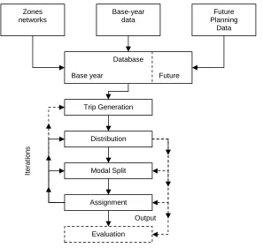
(23) Trip Generation. Veitch Lister Consulting. 5 Trip Generation Literature Review This chapter is the next part of the research and is basically considered reviewing the literature regarding trip generation. The chapter starts with an introduction to the first phase of the traditional four step model and attention is paid to the manner VLC classifies their model. Paragraph 5.5 and 5.6 describe the most common used approaches in trip generation: category analysis and regression analysis.. 5.1. Introduction. Trip generation modelling corresponds to the first stage of the conventional four step transport modelling theory, where the other stages are trip distribution, mode choice and traffic assignment to the transportation network. The purpose of the trip generation phase (e.g. production and attraction phase) in the ‘classical transport model’ is to predict the total person trips produced by and attracted to each zone in the study area based on social-economic information. The so called ‘classic transport model’ is a result of years of experimentation and development. As mentioned, the model consists of four stages and is depicted in figure 6 below:. Zones networks. Base-year data. Future Planning Data. Database Base year. Future. Trip Generation. Iterations. Distribution. Modal Split. Assignment Output Evaluation figure 6: Traditional 4-step Model. The approach starts by considering a zoning and network system, and the collection and coding of planning, calibration and validation data. These data would include base-year levels for population of different types in each zone of the study area as well as levels of economic activity including employment, shopping space, educational and recreational facilities. These data are then used to estimate a model of the total number of trips generated and attracted by each zone of the study area (trip generation) [Ortúzar and Willumsen., 2004]. This research project is focused on the development of trip generation equations with which a prediction of the total number of trips generated by origin (Oi) and attracted by destination (Dj) can be made. The focus of this research lies on the production stage of trip generation though. These models trip generation models can be further divided as home based, non-home based or work based trips. For the development of a good production-/attraction model it appears to be useful to make a classification of the trips by purpose, time of the day and person type. This will be discussed in. Van Beilen. 23. 2/8/2008.

(24) Trip Generation. Veitch Lister Consulting. paragraph 5.3. Subsequently, factors affecting trip generation and attraction are discussed and attention is paid to modeling approaches for production and attraction of trips. Most commonly used approaches in trip generation are regression-analysis and category-analysis which will be discussed in paragraph 5.5 and 5.6. Trip generation models can operate at different scales: zonal, household or person based. As well as the spatial scale, specific predictor variables also vary across regions and countries. Common predictors for production models are given in table 7. Variable Income Dwelling type Number of cars Household size Number of workers Number of dependents Racial/ethnic background. Type Continuous or ordinal Nominal Ordinal Continuous or ordinal Ordinal Ordinal Nominal. Sub-split. White / blue collar Split by age. table 7: Common predictors in trip production models. 5.2. Zones and networks. 5.2.1 Background A transport model is related to a certain study area. Displacements in this study area can start and finish on each address and travellers can make use of all kinds of transport. It is however impossible to collect and analyse data on the basis of individual data. A schematisation of reality is necessary. This schematisation includes the following components: • Area classification; the study area is classified into a number of zones. We study the displacements of and to each of these zones. All displacements are considered to start and finish in an imaginary point within this area, the centroid. • Networks; the transport system exists from a number of networks which represent the available transport modalities. Significant parameters are the number of applied zones and their dimension. Within the model the centroids are basically connected by connectors that represent the roads and their characteristics. Zones with a population from 1000 to 3000 people tend to satisfy well. Regarding the number of zones within a typical regional transport model, 300 to 500 zones is said to be reasonable. More than 1000 zones can be classified as extensive. All zones should be approximately equal in terms of dimension concerning traffic production. Furthermore one should aim for homogeneity towards land use within each zone [Immers & Stada, 1998]. The transport system is represented by a network of junctions and links. Characteristics of the network are ascribed to the links, for instance; length, speed and capacity. The junctions are not specially qualified. Networks tend to be more and more represented as multimodal network models where different ways of transport are connected mutually instead of separate networks for different modalities. A typical regional transport model consists of 1000 to 5000 junctions; over 10.000 junctions can be classified as extensive [Immers & Stada, 1998]. 5.2.2 VLC’s SEQ Transport model The household survey of the SEQ region consists of approximately 4200 Census Collection Districts (CCD) with approximately 225 households (which equals +/560 person) per CCD. It is not usually desirable to model the area with such an extensive number of zones since it will influence the complexity and dimension of the model. Based on geographical and demographical data the existing modelled area is figure 7: VLC's SEQ zoning Van Beilen. 24. 2/8/2008.

(25) Trip Generation. Veitch Lister Consulting. brought to 1529 zones with a total number of 1.101.164 households and a total population of 2.787.092 people. So each zone approximately contains 720 households and 1823 people. figure 7 depicts the zoning of the South East Queensland region as currently modeled by VLC which is pretty extensive. VLC’s zoning system also includes a significant “influence area”, also known as a buffer region. This area is included to better estimate travel patterns within the core study area, and minimize the “boundary effects”. For detailed modeling, VLC also utilizes a 5448 zone model, where each travel zone represents a CCD or smaller. In terms of transport infrastructure, VLC’s model of SEQ consists of approximately 20,000 junctions, and over 50,000 one-way link sections.. 5.3. Classification. Classification of trips according to Ortúzar and Willumsun is done by: trip purpose, time of day and by person type. 5.3.1 Trip purpose Ortúzar and Willumsun identify different trip purposes and model them separately to obtain better trip generation, trip distribution and mode choice models. In the case of home based trips, five categories are distinguished: • Trips to work • Trips to school or college (education trips); • Shopping trips; • Social and recreational trips; • Other trips; The first two are usually called compulsory trips and all the others are often optional trips. In the past, non-home based trips were often not separated because they only amounted to a small percentage (15% - 20%) of all trips [Ortúzar, 2004]. However, VLC research showed that the scale of non-home based travel is rapidly increasing, and as such, they will be considered as part of their trip generation model. The “QT_Overall_Purpose_DMR” column in the SEQTS_TRIPS table of the SEQTS Access database is a combination of the categories “QT End” and “QT Start” purposes to create a single purpose. Result is the following table 8, defining the possible overall trip purposes per person in the Household Travel Survery: QT_OVERALL_PURPOSE_DMR Home Based Work. Shopping Based Shopping. Home Based Education - Pre Primary. Shopping Based Other. Home Based Education - Secondary. Non Home/Work/Shopping Based. Home Based Education - Tertiary. Work Based Other. Home Based Other. Work Based Shopping. Home Based Shopping. Work Based Work. Home Based Social table 8: Overall trip purposes as in the SEQ household survey data. Veitch Lister Consulting distinguishes home based trip purpose categories and non-home based trip purpose categories as in table 9: VLC’s Trip Purpose Categories Home-Based Work: Blue Collar (HBW-Blue);. Shopping-Based Personal Business and Shopping (SBS);. Home-Based Work: White Collar (HBW-White);. Shopping-Based Other (SBO);. Home-Based Education: Pre and Primary School (HBE-PPrim);. Other Non-Home-Based Trips (ONHB);. Home-Based Education: Secondary School (HBE-Sec);. Work-Based Other (WBO);. Home-Based Education: Tertiary Institution (HBE-Ter);. Work-Based Shopping/Personal Business (WBS);. Home-Based Shopping/Personal Business (HBS);. Work-Based Work (WBW);. Home-Based Social/Recreational (HBR); Home-Based Other (HBO); table 9: VLC’s Trip purpose categories. Van Beilen. 25. 2/8/2008.

(26) Trip Generation. Veitch Lister Consulting. Else than Ortúzar states, VLC does take into account the non-home based trips separately, since it is presumed that the amount these trips is growing and currently attributes more than 15% – 20% of all trips. Furthermore we can read from the tables above that the available data as collected in the Household Travel Survey almost entirely corresponds with the VLC’s standard trip purpose categories. The main difference can be found in the home-based work purpose that is divided in blue collar and white collar work based trips, by VLC. Blue and white collar workers have been defined in terms of the following occupation classifications: Blue Collar Occupations • Tradespersons; • Plant and Machinery Operators; • Labourers and Administration. White Collar Occupations • Managerial and Administration; • Professional; • Para-Professional; • Clerical; • Sales and Personal Services. White Collar workers tend to be situated at an office mainly and exhibit different travel behavior to blue collar workers. Using this distinction means the available data has to be translated to VLC standards. This is done by reviewing the occupation of each household member within the travel survey data and adding an extra value(definition) to each member. The following occupations in table 10 appear from the survey data and are translated to the VLC definitions: CODE_DESCRIPTION N/A Missing Managers and Administrators Professionals Associate professionals Tradespersons Advanced Clerical and Service Workers Intermediate Clerical, Sales and Service Workers Intermediate Production and Transport Workers Elementary Clerical, Sales and Service Workers Labourers. VLC_DEFINITION White White White Blue White White Blue White Blue. table 10: SEQ Occupation descriptions specified to VLC definitions. If occupation data of a household member is N/A (not available) or missing these households were excluded entirely. As mentioned in paragraph 4.1.1 this was the case for 216 households. 5.3.2 By Time of Day Trips are often classified into peak and off-peak period trips; the proportion of journeys by different purposes usually varies greatly within time of day [Ortzúzar, 2004]. For this research we won’t classify trip generation by different times of the day and just take the daily data. This will actually be divided after the distribution phase in the four-step model. 5.3.3 By Person Type This is another important classification, as individual travel behaviour is heavily dependant on socioeconomic attributes. The following categories are usually employed: • Income level • Car ownership (typically three strata: 0, 1 and 2 or more cars); • Household size and structure (e.g. six strata in most British studies);. Van Beilen. 26. 2/8/2008.

(27) Trip Generation. Veitch Lister Consulting. It is important to note that the total number strata can increase very rapidly and this may have strong implications in terms of data requirements, model calibration and use, particularly when using category analysis [Ortuzar, 2004]. In terms of data preparation for trip production, VLC does not specifically classifies trips by person type.. 5.4. Factors affecting Trip Generation. Trip generation is on the one hand affected by production factors and on the other hand by attraction factors. Production factors are often based on household demographics and other socio economic factors whereas attraction factors tell us something about land use. 5.4.1 Factors affecting production The following factors have been proposed for consideration in many practical studies: • Income; • Car ownership; • Household structure; • Family size; • Value of land; • Residential density; • Accessibility; The first four have been considered in several trip generation studies, while value of land and residential density are typical of zonal studies. Accessibility has rarely been used although most studies have attempted to include it [Ortuzar, 2004]. Ignoring the accessibility factor in the model though, means production and attraction of a zone are insensible for changes in the transport system. This is a basic shortcoming of the existing model. Since accessibility definitely is an important factor for determining productions and attractions several models have been developed but there isn’t much accordance regarding the accuracy. Reason lays in the difficulty of quantifying the concept of accessibility [Immers & Stada, 1998]. In case of VLC’s trip production model there are seven “stratified household attribute groups” (see Appendix 2 for further detail) considered as production factors, defined as follows: - household size (1,2,3,4,5,6+) - car ownership (0,1,2,3+) - resident blue collar workers (0,1,2,3+) - resident white collar workers (0,1,2,3+) - resident (0-17); dependants (0,1,2,3,4+) - resident (18-64); dependants (0,1,2,3+) - resident (65+); dependants (0,1,2+) VLC classifies the “dependants” in aforementioned attribute groups since it is assumed that the different dependant groups cause different affects on trip generation. For example, the dependants aged 0-17 will mostly generate home based - education trips. As can be seen, income level does not play a direct roll within VLC’s current trip production model. This is due to the fact that income level and car ownership tend to be highly correlated, and VLC research has previously shown car ownership to be the more important variable. 5.4.2 Factors affecting attraction The following factors have been proposed to influence the attraction of a zone: • Employment • Land use o Industrial o Education o Commercial o Service industry (e.g. hospitals, banks, public institutions...) o Recreation (e.g. sport accommodations, sights and attractions...) o Storing and transfer (harbours, airports…) • Accessibility This research is basically focused on factors affecting production rather than the factors affecting attraction. So no further attention is paid to these factors at this stage and deserves further research in future modelling phases.. Van Beilen. 27. 2/8/2008.

No results found