Binarization of Synchronous Context Free Grammars

Liang Huang

USC/Information Science Institute

Hao Zhang

Daniel Gildea

Kevin Knight

USC/Information Science Institute

Systems based on synchronous grammars and tree transducers promise to improve the quality of statistical machine translation output, but are often very computationally intensive. The complexity is exponential in the size of individual grammar rules due to arbitrary re-orderings between the two languages. We develop a theory of binarization for synchronous context-free grammars and present a linear-time algorithm for binarizing synchronous rules when possible. In our large-scale experiments, we found that almost all rules are binarizable and the resulting binarized rule set significantly improves the speed and accuracy of a state-of-the-art syntax-based machine translation system. We also discuss the more general, and computationally more difficult, problem of finding good parsing strategies for non-binarizable rules, and present an approximate polynomial-time algorithm for this problem.

1. Introduction

Several recent syntax-based models for machine translation (Chiang 2005; Galley et al. 2004) can be seen as instances of the general framework of synchronous grammars and tree transducers. In this framework, both alignment (synchronous parsing) and decoding can be thought of as parsing problems, whose complexity is in general ex-ponential in the number of nonterminals on the right-hand side of a grammar rule. To alleviate this problem, we investigate bilingual binarization as a technique to fac-tor each synchronous grammar rule into a series of binary rules. Although mono-lingual context-free grammars (CFGs) can always be binarized, this is not the case

∗ Information Science Institute, 4676 Admiralty Way, Marina del Rey, CA 90292. E-mail: lhuang@isi.edu, liang.huang.sh@gmail.com.

∗∗ 1600 Amphitheatre Parkway, Mountain View, CA 94303. E-mail: haozhang@google.com.

† Computer Science Dept., University of Rochester, Rochester NY 14627. E-mail: gildea@cs.rochester.edu. ‡ Information Science Institute, 4676 Admiralty Way, Marina del Rey, CA 90292. E-mail: knight@isi.edu.

for all synchronous rules; we investigate algorithms for non-binarizable rules as well. In particular:

r

linear-timebinarization algorithm such that the resulting rule set allows efficient algorithms for both synchronous parsing and decoding with integratedn-gram language models.

r

translation quality on a large-scale Chinese-to-English syntax-based system, compared to a more typical baseline method, and a state-of-the-art phrase-based system.

r

sets, and show that the vast majority is binarizable. However, we also provide, for the first time, real examples of non-binarizable cases verified by native speakers.

r

problem of finding the most efficient synchronous parsing or decoding strategy for arbitrary synchronous context-free grammar (SCFG) rules, including non-binarizable cases. Although this problem is believed to be NP-complete, we prove two results that substantially reduce the search space over strategies. We also present an optimal algorithm that runs tractably in practice and a polynomial-time algorithm that is a good approximation of the former.

Melamed (2003) discusses binarization of multi-text grammars on a theoretical level, showing the importance and difficulty of binarization for efficient synchronous parsing. One way around this difficulty is to stipulate that all rules must be binary from the outset, as in Inversion Transduction Grammar (ITG) (Wu 1997) and the binary SCFG employed by the Hiero system (Chiang 2005) to model the hierarchical phrases. In contrast, the rule extraction method of Galley et al. (2004) aims to incorporate more syntactic information by providing parse trees for the target language and extracting tree transducer rules that apply to the parses. This approach results in rules with many nonterminals, making good binarization techniques critical.

We explain how synchronous rule binarization interacts with n-gram language models and affects decoding for machine translation in Section 2. We define binarization formally in Section 3, and present an efficient algorithm for the problem in Section 4. Experiments described in Section 51 _{show that binarization improves machine} trans-lation speed and quality. Some rules cannot be binarized, and we present a decoding strategy for these rules in Section 6. Section 7 gives a solution to the general theo-retical problem of finding optimal decoding and synchronous parsing strategies for arbitrary SCFGs, and presents complexity results on the nonbinarizable rules from our Chinese–English data. These final two sections are of primarily theoretical interest, as nonbinarizable rules have not been shown to benefit real-world machine translation sys-tems. However, the algorithms presented may become relevant as machine translation systems improve.

2. Motivation

Consider the following Chinese sentence and its English translation:

(1) 

B`aow¯eier

Powell

y ˇu

with ™™

Sh¯al´ong

Sharon >L

j ˇux´ıng

hold †

le

[past.]

hu`ıt´an

meeting “Powell held a meeting with Sharon”

Suppose we have the following SCFG, where superscripts indicate reorderings (formal definitions of SCFGs with a more flexible notation can be found in Section 3):

(2)

S → NP1 _PP2 _VP3_{, NP}1 _VP3 _PP2

NP → /B`aow¯eier, Powell

VP → >L † /j ˇux´ıng le hu`ıt´an, held a meeting

PP → ™™ /y ˇu Sh¯al´ong, with Sharon

Decoding can be cast as a (monolingual) parsing problem because we only need to parse the source-language side of the SCFG, as if we were constructing a CFG by projecting the SCFG onto its Chinese side:

(3)

S → NP PP VP

NP → /B`aow¯eier

VP → >L † /j ˇux´ıng le hu`ıt´an

PP → ™™ /y ˇu Sh¯al´ong

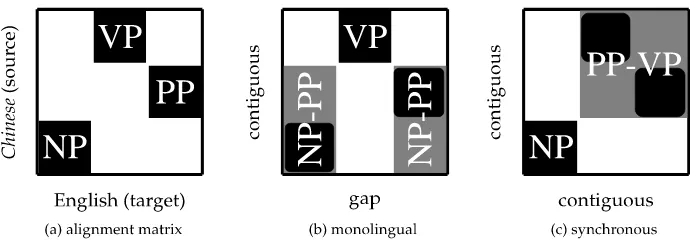
The only extra work we need to do for decoding is to build corresponding target-language (English) subtrees in parallel. In other words, we buildsynchronous trees when parsing the source-language input, as shown in Figure 1.

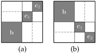
For efficient parsing, we need to binarize the projected CFG either explicitly into Chomsky Normal Form as required by the CKY algorithm, or implicitly into a dotted representation as in the Earley algorithm. To simplify the presentation, we will focus on the former, but the following discussion can be easily adapted to the latter. Rules can be binarized in different ways. For example, we could binarize the first rule left to right or right to left (see Figure 2):

S → NP-PP VP

NP-PP → NP PP or

S → NP PP-VP PP-VP → PP VP

We call these intermediate symbols (e.g., PP-VP)virtual nonterminalsand correspond-ing rulesvirtual rules, whose probabilities are all set to 1.

Figure 1

A pair of synchronous parse trees in the SCFG (2). The superscript symbols (¦?◦•_{) indicate pairs}

Figure 2

The alignment matrix and two binarization schemes, with virtual nonterminals in gray. (a) A two-dimensional matrix representation of the first SCFG rule in grammar 2. Rows are positions in Chinese: columns are positions in English, and black cells indicate positions linked by the SCFG rule. (b) This scheme groups NP and PP into an intermediate state which contains a gap on the English side. (c) This scheme groups PP and VP into an intermediate state which is contiguous on both sides.

These two binarizations are no different in the translation-model-only decoding described previously, just as in monolingual parsing. However, in the source-channel approach to machine translation, we need to combine probabilities from the translation model (TM) (an SCFG) with the language model (ann-gram), which has been shown to be very important for translation quality (Chiang 2005). To do bigram-integrated decoding (Wu 1996), we need to augment each chart item (X,i,j) with two target-languageboundary wordsuandvto produce a bigram-item which we denote Ãu···X v

i j !

.2 Now the two binarizations have very different effects. In the first case, we first com-bine NP with PP. This step is written as follows in the weighted deduction notation of Nederhof (2003):

µ

Powell ··· Powell

NP

1 2

¶

:p µ

with ··· Sharon

PP

2 4

¶

:q µ

Powell···Powell ··· with···Sharon

NP-PP

1 4

¶

:pq

wherepandqare the scores of antecedent items.

This situation is unpleasant because in the target language NP and PP are not

contiguous so we cannot apply language model scoring when we build the NP-PP item. Instead, we have to maintain all four boundary words (rather than two) and postpone the language model scoring till the next step where NP-PP is combined withÃheld···meeting

VP 2 4

!

to form an S item. We call this binarization methodmonolingual binarizationbecause it works only on the source-language projection of the rule without respecting the constraints from the other side.

This scheme generalizes to the case where we have n nonterminals in a SCFG rule, and the decoder conservatively assumes nothing can be done on language model scoring (because target-language spans are non-contiguous in general) until the real nonterminal has been recognized. In other words, target-language boundary words

from each child nonterminal of the rule will be cached in all virtual nonterminals derived from this rule. In the case ofm-gram integrated decoding, we have to maintain 2(m−1) boundary words for each child nonterminal, which leads to a prohibitive over-all complexity ofO(|w|3+2n(m−1)_{), which is exponential in rule size (Huang, Zhang, and} Gildea 2005). Aggressive pruning must be used to make it tractable in practice, which in general introduces many search errors and adversely affects translation quality.

In the second case, however, we have:

µ

with ··· Sharon

PP

2 4

¶

:r µ

held ··· meeting

VP

4 7

¶

:s µ

held ··· Sharon

PP-VP

2 7

¶

:rs·Pr(with|meeting)

Here, because PP and VP are contiguous (but swapped) in the target language, we can include the language model score by multiplying in Pr(with|meeting), and the resulting item again has two boundary words. Later we multiply in Pr(held|Powell) when the resulting item is combined withµPowell···Powell

NP 1 2

¶

to form an S item. As illustrated in Figure 2, PP-VP has contiguous spans on both source- and target-sides, so that we can generate a binary-branching SCFG:

(4) S → NP

1 _PP-VP2_{, NP}1 _PP-VP2

PP-VP → VP1 _PP2_{, PP}2 _VP1

In this casem-gram integrated decoding can be done inO(|w|3+4(m−1)_{) time, which is a} much lower-order polynomial and no longer depends on rule size (Wu 1996), allowing the search to be much faster and more accurate, as is evidenced in the Hiero system of Chiang (2005), which restricts the hierarchical phrases to form binary-branching SCFG rules.

Some recent syntax-based MT systems (Galley et al. 2004) have adopted the for-malism of tree transducers (Rounds 1970), modeling translation as a set of rules for a transducer that takes a syntax tree in one language as input and transforms it into a tree (or string) in the other language. The same decoding algorithms are used for machine translation in this formalism, and the following example shows that the same issues of binarization arise.

Suppose we have the following transducer rules:

(5)

S(x1:NPx2:PPx3:VP) → S(x1 VP(x3x2))

NP( /B`aow¯eier) → NP(NNP(Powell))

VP(>L † /j ˇux´ıng le hu`ıt´an) → VP(VBD(held) NP(DT(a) NPS(meeting)))

PP( ™™ /y ˇu Sh¯al´ong) → PP(TO(with) NP(NNP(Sharon)))

where the reorderings of nonterminals are denoted by variables xi. In the

Figure 3

Two equivalent representations of the first rule in Example (5): (a) tree transducer; (b) Synchronous Tree Subsitution Grammar (STSG). The↓arrows denote substitution sites, which correspond to variables in tree transducers.

nonterminal for each right-hand-side tree, we can convert the transducer representation to an SCFG with the same generative capacity. We can again create a projected CFG which will be exactly the same as in Example (3), and build English subtrees while parsing the Chinese input. In this sense we can neglect the tree structures when binarizing a tree-transducer rule, and consider only the alignment (or permutation) of the nonterminal variables. Again, rightmost binarization is preferable for the first rule.

In SCFG-based frameworks, the problem of finding a word-level alignment be-tween two sentences is an instance of the synchronous parsing problem: Given two strings and a synchronous grammar, find a parse tree that generates both input strings. The benefit of binary grammars also applies in this case. Wu (1997) shows that parsing a binary-branching SCFG is in O(|w|6_{), while parsing SCFG with arbitrary rules is} NP-hard (Satta and Peserico 2005). For example, in Figure 2, the complexity of syn-chronous parsing for the original grammar (a) isO(|w|8_{), because we have to maintain} four indices on either side, giving a total of eight; parsing the monolingually binarized grammar (b) involves seven indices, three on the Chinese side and four on the En-glish side. In contrast, the synchronously binarized version (c) requires only 3 + 3 = 6 indices, which can be thought of as “CKY in two dimensions.” An efficient alignment algorithm is guaranteed if a binarization is found, and the same binarization can be used for decoding and alignment. We show how to find optimal alignment algorithms for non-binarizable rules in Section 7; in this case different grammar factorizations may be optimal for alignment and for decoding with n-gram models of various orders. Handling difficult rules may in fact be more important for alignment than for decoding, because although we may be able to find good translations during decoding within the space permitted by computationally friendly rules, during alignment we must handle the broader spectrum of phenomena found in real bitext data.

In general, if we are given an arbitrary synchronous rule with many nonterminals, what are the good decompositions that lead to a binary grammar? Figure 2 suggests that a binarization is good if every virtual nonterminal has contiguous spans on both sides. We formalize this idea in the next section.

3. Synchronous Binarization Definition 1

A synchronous CFG (SCFG) is a context-free rewriting system for generating string pairs. Each rule (synchronous production)

rewrites a pair ofsynchronous nonterminals(A,B) in two dimensions subject to the constraint that there is a one-to-one mapping between the nonterminal occurrences inα

and the nonterminal occurrences inβ. Each co-indexed child nonterminal pair is a pair of synchronous nonterminals and will be further rewritten as a unit.

Note that this notation, due to Satta and Peserico (2005), is more flexible than those in the previous section, in the sense that we can allow different symbols to be synchro-nized, which is essential to capture the syntactic divergences between languages. For example, the following rule from Chinese to English

(6) VP→VB1 _NN2_{, VP→VBZ}1 _NNS2

illustrates the fact that Chinese does not have a plural noun (NNS) or third-person-singular verb (VBZ), although we can always convert this form back into the other notation by creating a compound nonterminal alphabet:

(VP, VP)→(VB, VBZ)1 _{(NN, NNS)}2_{, (VB, VBZ)}1 _{(NN, NNS)}2_.

We define the languageL(G) produced by an SCFGGas the pairs of terminal strings produced by rewriting exhaustively from the start nonterminal pair.

As shown in Section 4.2, terminals do not play an important role in binarization. So we now write rules in the following notation:

X→X1 1 ...X

n

n , Y→Y

π(1)

π(1)...Y

π(n)

π(n)

whereXiandYiare variables ranging over nonterminals in the source and target

pro-jections of the synchronous grammar, respectively, andπis thepermutationof the rule. For example, in rule (6), we haven=2, X=Y=VP,X1=VB,X2=NN,Y1 =VBZ, Y2=NNS, andπis the identity permutation. Note that this general notation includes cases where a nonterminal occurs more than once in the right-hand side, for example, whenn=2, X=Y=A, andX1=X2 =Y1=Y2=B, we can have the following two rules:

A→B1

B2

, A→B2

B1 ;

A→B1

B2

, A→B1

B2_.

We also define an SCFG rule as n-ary if its permutation is ofn and call an SCFG

n-ary if its longest rule isn-ary. Our goal is to produce an equivalentbinarySCFG for an inputn-ary SCFG.

However, not every SCFG can be binarized. In fact, the binarizability of an n -ary rule is determined by the structure of its permutation, which can sometimes be resistant to factorization (Aho and Ullman 1972). We now turn to rigorously defining the binarizability of permutations.

Definition 2

For example, (3, 5, 4) is a permuted sequence whereas (2, 5) is not. As special cases, single numbers are permuted sequences as well. (3; 5, 4) is a proper split of (3, 5, 4) whereas (3, 5; 4) is not. A proper split has the following property:

Lemma 1

For a permuted sequencea,a=(b;c) is a proper split if and only ifb<corc<b. Proof

The⇒direction is trivial by the definition of proper split.

We prove the ⇐ direction by contradiction. Ifb<c butb is not a permuted se-quence, i.e., the set of b’s elements is not consecutive, then there must be somex∈c such that minb<x<maxb, which contradicts the fact thatb<c. We have a similar contradiction if cis not a permuted sequence. Now that both b and care permuted sequences, (b;c) is a proper split. The case whenb>cis similar.¥

Definition 3

A permuted sequenceais said to bebinarizableif either 1. ais a singleton, that is,a=(a), or

2. there is a proper splita=(b;c) wherebandcare both binarizable. We call such split abinarizable split.

This is a recursive definition, and it implies that there is a hierarchical binarization pattern associated with each binarizable sequence, which we now rigorously define.

Definition 4

Abinarization treebi(a) of a binarizable sequenceais either 1. aifa=(a), or

2. [bi(b),bi(c)] ifb<c, orhbi(b),bi(c)iotherwise, wherea=(b;c) is a binarizable split, andbi(b) is a binarization tree ofbandbi(c) a binarization tree ofc.

Here we use [] andhifor straight (b<c) and inverted (b>c) combinations, respec-tively, following the ITG notation of Wu (1997). Note that a binarizable sequence might have multiple binarization trees. See Figure 4 for a binarizable sequence (1, 2, 4, 3) with its two possible binarization trees and a non-binarizable sequence (2, 4, 1, 3).

We are now able to define the binarizability of SCFGs:

Definition 5

An SCFG is said to bebinarizableif the permutation of each synchronous production is binarizable. We denote the class of binarizable SCFGs asbSCFG.

Figure 4

(a)–(c) Alignment matrix and two binarization trees for the permutation sequence (1, 2, 4, 3). (d) Alignment matrix for the non-binarizable sequence (2, 4, 1, 3).

Figure 5

Subclasses of SCFG. The thick arrow denotes the direction of synchronous binarization and indicates bSCFG can collapse to binary SCFG.

decomposes the original permutation into a set of binary ones. All that remains is to decorate the skeleton binarization tree with nonterminal symbols and attach terminals to the skeleton appropriately (see the next section for details). We state this result as the following theorem:

Theorem 1

For each grammarGin bSCFG, there exists a binary SCFGG0_{, such thatL(G}0_)=L(G).

4. Binarization Algorithms

We have reduced the problem of binarizing an SCFG rule into the problem of binarizing its permutation. The simplest algorithm for this problem is to try all bracketings of a permutation and pick one that corresponds to a binarization tree. The number of all possible bracketings of a sequence of length n is known to be the Catalan Number (Catalan 1844)

Cn= 1

n+1

µ

2n n

¶

Another problem besides efficiency is that there are possibly multiple binarization trees for many permutations whereas we just need one. We would prefer aconsistent

pattern of binarization trees across different permutations so that sub-binarizations (vir-tual nonterminals) can be shared. For example, permutations (1, 3, 2, 5, 4) and (1, 3, 2, 4) can share the common sub-binarization tree [1,h3, 2i]. To this end, we can borrow the non-ambiguous ITG of Wu (1997, Section 7) that prefers left-heavy binarization trees so that for each permutation there is a unique synchronous derivation.3_{We now refine the} definition of binarization trees accordingly.

Definition 6

A binarization treebi(a) is said to becanonicalif the split at each non-leaf node of the tree is therightmostbinarizable split.

For example, for sequence (1, 2, 4, 3), the binarization tree [[1, 2],h4, 3i] is canonical, whereas [1, [2,h4, 3i]] is not, because its top-level split is not at the rightmost binarizable split (1, 2; 4, 3). By definition, there is a unique canonical binarization tree for each binarizable sequence.

We next present an algorithm that is both fast and consistent.

4.1 The Linear-Time Skeleton Algorithm

Shapiro and Stephens (1991, page 277) informally present an iterative procedure that, in each pass, scans the permuted sequence from left to right and combines two adja-cent subsequences whenever possible. This procedure produces canonical binarization trees and runs inO(n2) time because we neednpasses in the worst case. Inspired by the Graham Scan Algorithm (Graham 1972) for computing convex hulls from computa-tional geometry, we modify this procedure and improve it into a linear-time algorithm that only needs one pass through the sequence.

The skeleton binarization algorithm is an instance of the widely used left-to-right shift-reduce algorithm. It maintains a stack for contiguous subsequences discovered so far; for example: 2–5, 1. In each iteration, it shifts the next number from the input and repeatedly tries to reduce the top two elements on the stack if they are consecutive. See Algorithm 1 for the pseudo-code and Figures 6 and 7 for example runs on binarizable and non-binarizable permutations, respectively.

We need the following lemma to prove the properties of the algorithm:

Lemma 2

Ifcis a permuted sequence (properly) within a binarizable permuted sequencea, then cis also binarizable.

Proof

We prove by induction on the length ofa. Base case:|a|=2, a (proper) subsequence of a, has length 1, so it is binarizable. For|a|>2, becausea has a binarization tree, there

Algorithm 1The linear-time binarization algorithm. 1: functionSYNCHRONOUSBINARIZER(π)

2: top←0 .stack top pointer

3: PUSH(stack, (π(1),π(1))) .initial shift

4: fori←2to|π|do .for each remaining element

5: PUSH(stack, (π(i),π(i))) .shift

6: whiletop>1andCONSECUTIVE(stack[top],stack[top−1])do

7: .keep reducing if possible

8: (p,q)←COMBINE(stack[top],stack[top−1])

9: top←top−2

10: PUSH(stack, (p,q))

11: return(top=1) .returns true iff. the input is reduced to a single element

12:

13: functionCONSECUTIVE((a,b), (c,d))

14: return(b=c−1)or(d=a−1) .either straight or inverted

15: functionCOMBINE((a,b), (c,d))

16: A={min(a,c)...max(b,d)} 17: B={a...b}

18: C={c...d} 19: rule[A]=A→ B C 20: return(min(a,c),max(b,d))

Figure 6

Example of Algorithm 1 on the binarizable input (1, 5, 3, 4, 2). The rightmost column shows the binarization-trees generated at each reduction step.

exists a (binarizable) split which is nearest to the root and splitscinto two parts. Let the split be (b1,c1;c2,b2), wherec=(c1;c2), and eitherb1orb2can be empty. By Lemma 1, we havec1<c2orc1 >c2. By Lemma 1 again, we have that (c1;c2) is a proper split ofc, i.e., bothc1andc2are themselves permuted sequences. We also know both (b1,c1) and (c2,b2) are binarizable. By the induction hypothesis,c1 andc2are both binarizable. So we conclude thatc=(c1;c2) is binarizable (See figure 8).¥

We now state the central result of this work.

Theorem 2

Figure 7

Example of Algorithm 1 on the non-binarizable input (2, 5, 4, 1, 3).

Figure 8

Illustration of the proof of Lemma 2. The arrangement of (b1,c1;c2,b2) must be either all straight as in (a) or all inverted as in (b).

Proof

We prove the following three parts of this theorem:

1. If Algorithm 1 succeeds, thenais binarizable because we can recover a binarization tree from the algorithm.

2. Ifais binarizable, then Algorithm 1 must succeed and the binarization tree recovered must be canonical:

We prove by a complete induction onn, the length ofa. Base case:n=1, trivial. Assume it holds for alln0<n.

Ifais binarizable, then leta=(b;c) be its rightmost binarizable split. By definition, bothbandcare binarizable. By the induction hypothesis, the algorithm succeeds on the partial inputb, reducing it to the single element

Figure 9

Illustration of the proof of Theorem 2. The combination of (b;c1) (in dashed squares) contradicts the assumption that (b;c) is the rightmost binarizable split ofa.

Therefore, the algorithm will scan through the wholecas iffrom the empty stack. By the induction hypothesis again, it will reducecintostack[1] on the stack and recover its canonical binarization treebi(c). Becausebandc are combinable, the algorithm reducesstack[0] andstack[1] in the last step, forming the canonical binarization tree fora, which is either [bi(b),bi(c)] or hbi(b),bi(c)i.

3. The running time of Algorithm 1 (regardless of success or failure) is linear inn:

By amortized analysis (Cormen, Leiserson, and Rivest 1990), there are exactlynshifts and at mostn−1 reductions, and each shift or reduction takesO(1) time. So the total time complexity isO(n).

¥

4.2 Dealing with Terminals and Adapting to Tree Transducers

Thus far we have discussed how to binarize synchronous productions involving only nonterminals through binarizing the corresponding skeleton permutations. We now turn to technical details for the implementation of a synchronous binarizer in real MT systems. We will first show how to deal with the terminal symbols, and then describe how to adapt it to tree transducers.

Consider the following SCFG rule:

(7) ADJP → RB1 _{#/f `uz´ePP}2 _„/deNN3_, ADJP → RB1 _{responsible for the NN}3 _PP2

whose permutation is (1, 3, 2). We run the skeleton binarization algorithm and get the (canonical) binarization tree [1,h3, 2i], which corresponds to [RB,hNN, PPi] (see Figure 10(a)). The alignment matrix is shown in Figure 11.

We will then do a post-order traversal of the skeleton tree, and attach the terminals from both languages when appropriate. It turns out we can do this quite freely as long as we can uniquely reconstruct the original rule from its binary parse tree. We use the following rules for this step:

Figure 10

Attaching terminals in SCFG binarization. (a) The skeleton binarization tree, (b) attaching Chinese words at leaf nodes, (c) attaching English words at internal nodes.

Figure 11

Alignment matrix of the SCFG rule (7). Areas shaded in gray and light gray denote virtual nonterminals (see rules in Example (8)).

(except for the initial ones which are attached to the nonterminal on their right).

2. Attach target-language terminals to the internal nodes (virtual

nonterminals) of the skeleton tree. These terminals are attached greedily: When combining two nonterminals, all target-side terminal strings neighboring either nonterminal will be included. This greedy merging is motivated by the idea that the language model score helps to guide the decoder and should be computed as early as possible.

For example, at the leaf nodes, the Chinese word#/f `uz´e is attached to RB1 , and „/deto PP1 _{(Figure 10(b)). Next, when combining NN}3 _{and the virtual nonterminal} PP-„/de, we also include the English-side stringresponsible for the (Figure 10(c)). In order to do this rigorously we need to keep track of sub-alignments including both aligned nonterminals and incorporated terminals. A pre-order traversal of the fully decorated binarization tree gives us the following binary SCFG rules:

(8)

ADJP → V11 V22, ADJP → V11 V22

V1 → RB1 #/f `uz´e, V1 → RB1

V2 → V31 NN2, V2 → responsible for the NN2 V31

where the virtual nonterminals (illustrated in Figure 11) are:

V1: RB-#/f `uz´e

V2:hresp. for the NN, PP-„/dei V3: PP-„/de

Analogous to the “dotted rules” in Earley parsing for monolingual CFGs, the names we create for the virtual nonterminals reflect the underlying sub-alignments, ensuring intermediate states can be shared across different string-to-tree rules without causing ambiguity.

The whole binarization algorithm still runs in time linear in the number of symbols in the rule (including both terminals and nonterminals).

We now turn to tree transducer rules. We view each left-hand side subtree as a monolithic nonterminal symbol and factor each transducer rule into two SCFG rules: one from the root nonterminal to the subtree, and the other from the subtree to the leaves. In this way we can uniquely reconstruct the transducer derivation using the two-step SCFG derivation. For example, consider the following tree transducer rule:

We create a specific nonterminal, say, T859, which uniquely identifies the left-hand side subtree. This gives the following two SCFG rules:

ADJP → T859 1, ADJP → T859 1

T859 → RB1 #/f `uz´ePP2 „/deNN3, T859 → RB1 resp. for the NN3 PP2

The newly created nonterminals ensure that the newly created rules can only combine with one another to reconstruct the original rule, leaving the output of the transducer, as well as the probabilities it assigns to transductions, unchanged. The problem of binarizing tree transducers is now reduced to the binarization of SCFG rules, which we solved previously.

5. Experiments

In this section, we investigate two empirical questions with regard to synchronous binarization.

5.1 How Many Rules are (Synchronously) Binarizable?

(see Figure 12). However, for machine translation, the percentage of synchronous rules that are binarizable is what we care about. We answer this question in both large-scale automatically aligned data and small-scale hand-aligned data.

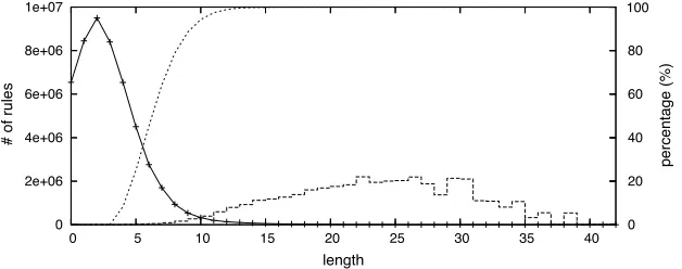
Automatically Aligned Data.Our rule set here is obtained by first doing word alignment using GIZA++ on a Chinese–English parallel corpus containing 50 million words in English, then parsing the English sentences using a variant of the Collins parser, and finally extracting rules using the graph-theoretic algorithm of Galley et al. (2004). We did a spectrum analysis on the resulting rule set with 50,879,242 rules. Figure 12 shows how the rules are distributed against their lengths (number of nonterminals). We can see that the percentage of non-binarizable rules in each bucket of the same length does not exceed 25%. Overall, 99.7% of the rules are binarizable. Even for the 0.3% of rules that are not binarizable, human evaluations show that the majority are due to alignment errors. Because the rule extraction process looks for rules that are consistent with both the automatic parses of the English sentences, and automatic word level alignments from GIZA++, errors in either parsing or word-level alignment can lead to noisy rules being input to the binarizer. It is also interesting to know that 86.8% of the rules have monotonic permutations, i.e., either taking identical or totally inverted order.

5.2 Hand-Aligned Data

One might wonder whether automatic alignments computed by GIZA++ are system-atically biased toward or against binarizability. If syntactic constraints not taken into account by GIZA++ enforce binarizability, automatic alignments could tend to contain spurious non-binarizable cases. On the other hand, simply by preferring monotonic alignments, GIZA++ might tend to miss complex non-binarizable patterns. To test this, we carried out experiments on hand-aligned sentence pairs with three language pairs: Chinese–English, French–English, and German–English.

Chinese–English Data.For Chinese–English, we used the data of Liu, Liu, and Lin (2005) which contains 935 pairs of parallel sentences. Of the 13,713 rules extracted using the same method described herein, 0.3% (44) are non-binarizable, which is exactly the

Figure 12

same ratio as the GIZA-aligned data. The following is an interesting example of non-binarizable rules:

where ... inwith ... Mishirais the long phrase in shadow modifyingMishira. Here the non-binarizable permutation is (3, 2, 5, 1, 4), which is reducible to (2, 4, 1, 3). The SCFG version of the tree-transducer rule is as follows:

where we indicate dependency links in solid arcs and permutation in dashed lines. It is interesting to examine dependency structures, as some authors have argued that they are more likely to generalize across languages than phrase structures. The Chinese ADVP1 _S)

/d¯angti¯an(lit.,that day) is translated into an English PP1

(on the same day), but the dependency structures on both sides are isomorphic (i.e., this is an extremely literal translation).

A simpler but slightly non-literal example is the following:

(10) ... ... ...

Û e1 j`ıny¯ıb `u

further [1

ji `u

on

-zh¯ongd¯ong

Mideast q:

w¯eij¯ı

crisis

]2 >L3 j ˇux´ıng

hold

4 hu`ıt´an

talk ... hold3 further1 talks4 [on the Mideast crisis]2

where the SCFG version of the tree-transducer rule (in the same format as the previous example) is:

Note that the Chinese ADVP1 _{Û e}

/j`ıny¯ıb `umodifying the verb VB3

becomes a JJ1 _{(further) in the English translation modifying the object of the verb, NNS}4_{, and} this change also happens to PP2_{. This is an example of syntactic divergence, where the} dependency structures are not isomorphic between the two languages (Eisner 2003).

and Chinese.” Our empirical results not only confirm that this is largely correct (99.7% in our data sets), but also provide, for the first time, “real examples” between English and Chinese, verified by native speakers. It is interesting to note that our non-binarizable examples include both cases of isomorphic and non-isomorphic dependency structures, indicating that it is difficult to find any general linguistic explanation that covers all such examples. Wellington, Waxmonsky, and Melamed (2006) used a different measure of non-binarizability, which is on the sentence-level permutations, as opposed to rule-level permutation as in our case, and reported 5% non-binarizable cases for a different hand-aligned English–Chinese data set, but they did not provide real examples.

French–English Data.We analyzed 447 hand-aligned French–English sentences from the NAACL 2003 alignment workshop (Mihalcea and Pederson 2003). We found only 2 out of 2,659 rules to be non-binarizable, or 0.1%. One of these two is an instance of topicalization:

The second instance is due to movement of an adverbial:

German–English Data. We analyzed 220 sentences from the Europarl corpus, hand-aligned by a native German speaker (Callison-Burch, personal communication). Of 2,328 rules extracted, 13 were non-binarizable, or 0.6%. Some cases are due to separable German verb prefixes:

Here the German prefix auf is separated from the verb auffordern (request). Another cause of non-binarizability is verb-final word order in German in embedded clauses:

English and French–English data. The results on binarizability of hand-aligned data for the three language pairs are summarized in Table 1.

It is worth noting that for most of these non-binarizable examples, there do exist alternative translations that only involve binarizable permutations. For example, in Chinese–English Example (9), we can move the English PPon the same dayto the first position (before will), which results in a binarizable permutation (1, 3, 2, 5, 4). Simi-larly, we can avoid non-binarizability in French–English Example (12) by moving the English adverbialstill under private ownership to the third position. German–English Example (13) would also become binarizable by replacingcall on with a single word

request on the English side. However, the point of this experiment is to test the ITG hypothesis by attempting toexplainexisting real data (the hand-aligned parallel text), rather than togeneratefresh translations for a given source sentence, which is the topic of the subsequent decoding experiment. This subsection not only provides the first solid confirmation of the existence of linguistically-motivated non-binarizable reorderings, but also motivates further theoretical studies on parsing and decoding with these non-binarizable synchronous grammars, which is the topic of Sections 6 and 7.

5.3 Does Synchronous Binarization Help Decoding?

We did experiments on our CKY-based decoder with two binarization methods. It is the responsibility of the binarizer to instruct the decoder how to compute the language model scores from children nonterminals in each rule. The baseline method is mono-lingual left-to-right binarization. As shown in Section 2, decoding complexity with this method is exponential in the size of the longest rule, and because we postpone all the language model scorings, pruning in this case is also biased.

To move on to synchronous binarization, we first did an experiment using this baseline system without the 0.3% of rules that are non-binarizable and did not observe any difference in BLEU scores. This indicates that we can safely focus on the binarizable rules, discarding the rest.

The decoder now works on the binary translation rules supplied by an external synchronous binarizer. As shown in Section 1, this results in a simplified decoder with a polynomial time complexity, allowing less aggressive and more effective pruning based on both translation model and language model scores.

We compare the two binarization schemes in terms of translation quality with various pruning thresholds. The rule set is that of the previous section. The test set has 116 Chinese sentences of no longer than 15 words, taken from the NIST 2002 test set. Both systems use trigram as the integrated language model. Figure 13 demonstrates that decoding accuracy is significantly improved after synchronous binarization. The number of edges (or items, in the deductive parsing terminology) proposed during

Table 1

Summary of non-binarizable ratios from hand-aligned data.

Sentence Non-Binarizable

Language Pair Pairs Rules Rules Major Causes for Non-Binarization

Figure 13

Comparing the two binarization methods in terms of translation quality against search effort.

Table 2

Machine translation results for syntax-based systems vs. the phrase-based Alignment Template System.

System BLEU

monolingual binarization 36.25 synchronous binarization 38.44

alignment-template system 37.00

decoding is used as a measure of the size of search space, or time efficiency. Our system is consistently faster and more accurate than the baseline system.

We also compare the top result of our synchronous binarization system with the state-of-the-art alignment-template system (ATS) (Och and Ney 2004). The results are shown in Table 2. Our system has a promising improvement over the ATS system, which is trained on a larger data set but tuned independently. A larger-scale system based on our best result performs very well in the 2006 NIST MT Evaluation (ISI Machine Translation Team 2006), achieving the best overall BLEU scores in the Chinese-to-English track among all participants.4_{The readers are referred to Galley et al. (2004)} for details of the decoder and the overall system.

6. One-Sided Binarization

In this section and the following section, we discuss techniques for handling rules that are not binarizable. This is primarily of theoretical interest, as we found that they constitute a small fraction of all rules, and removing these did not affect our Chinese-to-English translation results. However, non-binarizable rules are shown to be important in explaining existing hand-aligned data, especially for other language pairs such as German–English (see Section 5.2, as well as Wellington, Waxmonsky, and Melamed [2006]). Non-binarizable rules may also become more important as machine translation

4 NIST 2006 Machine Translation Evaluation Official Results: see

Table 3

A summary of the four factorization algorithms, and the “incremental relaxation” theme of the whole paper. Algorithms 2–4 are for non-binarizable SCFGs, and are mainly of theoretical interest. Algorithms 1–3 make fewer and fewer assumptions on the strategy space, and produce parsing strategies closer and closer to the optimal. Algorithm 4 further improves Algorithm 3.

Section Algorithm Assumptions of Strategy Space Complexity

3–4 Alg. 1 (synchronous) Contiguous on both sides O(n) 6 Alg. 2 (one-sided, CKY) Contiguous on one side O(n3₎

7.2 Alg. 3 (optimal) No assumptions O(3

n₎

⇒Alg. 4 (best-first) O(9k_n2k₎

systems improve. Synchronous grammars that go beyond the power of SCFG (and therefore binary SCFG) have been defined by Shieber and Schabes (1990) and Rambow and Satta (1999), and motivated for machine translation by Melamed (2003), although previous work has not given algorithms for finding efficient and optimal parsing strate-gies for general SCFGs, which we believe is an important problem.

In the remainder of this section and the next section, we will present a series of algorithms that produce increasingly faster parsing strategies, by gradually relaxing the strong “continuity” constraint made by the synchronous binarization technique. As that technique requires continuity onboth languages, we will first study a relaxation where binarized rules are always continuous in one of the two languages, but may be discontinuous in the other. We will present a CKY-style algorithm (Section 6.2) for finding the best parsing strategy under this new constraint, which we callone-sided binarization. In practice, this factorization has the advantage that we need to maintain only one set of language model boundary words for each partial hypothesis.

We will see, however, that it is not always possible to achieve the best asymptotic complexity within this constraint. But most importantly, as the synchronous binariza-tion algorithm covers most of the SCFG rules in real data, the one-sided binarizabinariza-tion we discuss in this section is able to achieve optimal parsing complexity for most of the non-binarizable rules in real data. So this section can be viewed as a middle step between the synchronous binarization we focus on in the previous sections and the optimal factorization coming in Section 7, and also a trade-off point between simplicity and asymptotic complexity for parsing strategies of SCFGs. Table 3 summarizes this incremental structure of the whole paper.

6.1 Formalizing the Problem

The complexity for decoding given a grammar factorization can be expressed in terms of the number of spans of the items being combined at each step. As an example, Figure 14 shows the three combination steps for one factorization of the non-binarizable rule:

X→A1

B2

C3

D4

, X→B2

D4

A1

C3

(15)

Figure 14

The tree at the top of the figure defines a three-step decoding strategy for rule (15), building an English output string on the horizontal axis as we process the Chinese input on the vertical axis. In each step, the two subsets of nonterminals in the inner marked spans are combined into a new chart item with the outer spans. The intersection of the outer spans, shaded, has now been processed.

pair{A,B}must record a total of four string indices: positionsy1,y2,y3, andy4 in the Chinese string.

Any combination of two subsets of the rule’s nonterminals involves the indices for the spans of each subset. However, some of the indices are tied together: If we are joining two spans into one span in the new item, one of the original spans’ end-points must be equal to another span’s beginning point. For example, the indexy2 is the end-point of Ain Chinese, as well as the beginning position ofD. In general, if we are combining a subsetBof nonterminals havingbspans with a subsetChavingcspans, to produce a

spans for a combined subsetA=B∪C, the number of linked indices isb+c−a. In the example of the first step of Figure 14, subset{A}has two spans (one in each language) so b=1, and {B} also has two spans, soc=1. The combined subset {A,B}has two spans, soa=2. The total number of indices involved in a combination of two subsets is

2(b+c)−(b+c−a)=a+b+c (16)

where 2(b+c) represents the original beginning and end points, and b+c−a the number of shared indices. In the first step of Figure 14,a+b+c=1+1+2=4 total indices, and therefore the complexity of this step isO(|w|4_{) where|w|is the length of the} input Chinese strings, and we ignore the language model for the moment. Applying this formula to the second and third step, we see that the second isO(|w|5_{), and the} third is againO(|w|4_).

Algorithm 2AnO(n3_{) CKY-style algorithm for parsing strategies, keeping continuous} spans in one language. Takes an SCFG rule’s permutation as input and returns the complexity of the best parsing strategy found.

1: functionBESTCONTINUOUSPARSER(π)

2: n=|π|

3: forspan←1ton−1do 4: fori←1ton−spando 5: A={i...i+span} 6: best[A]=∞

7: forj←i+1toi+spando 8: B={i...j−1}

9: C={j...i+span}

10: Letaπ,bπ, andcπdenote the number ofπ(A),π(B), andπ(C)’s spans

11: compl[A→ B C]=max{aπ+bπ+cπ, best[B], best[C]}

12: ifcompl[A→ B C]<best[A]then

13: best[A]=compl[A→ B C]

14: rule[A]=A→ B C

15: returnbest[{1...n}]

the diagram has three indices into the English string, so the complexity of the first step isO(|w|4+3_)=O(|w|7_{), the second step isO(|w|}8_{), and the third is againO(|w|}7_).

6.2 A CKY-Style Algorithm for Parsing Strategies

TheO(n3_{) algorithm we present in this section can find good factorizations for most} non-binarizable rules; we discuss optimal factorization in the next section. This algorithm, shown in Algorithm 2, considers only factorizations that have only one span in one of the two languages, and efficiently searches over all such factorizations by combining adjacent spans with CKY-style parsing.5_{The input is an SCFG grammar} rule in its abstract form, which is a permutation, andbestis a dynamic programming table used to store the lowest complexity with which we can parse a given subset of the input rule’s child nonterminals.

Although this CKY-style algorithm finds the best grammar factorization maintain-ing continuous spans in one of the two dimensions, in general the best factorization may require discontinuous spans in both dimensions. As an example, the following pattern causes problems for the algorithm regardless of which of the dimensions it parses across:

1↔ 1 n/2+1↔ 2

2↔n/2+1 n/2+2↔n/2+2

3↔ 3 n/2+3↔ 4

4↔n/2+3 n/2+4↔n/2+4

... ...

This pattern, shown graphically in Figure 15 forn=16, can be parsed in timeO(|w|10₎ by maintaining a partially completed item with two spans in each dimension, one

Figure 15

Left, a general pattern of non-binarizable permutations. Center, a partially completed chart item with two spans in each dimension; the intersection of the completed spans is shaded. Right, the combination of the item from the center panel with a singleton item. The two subsets of nonterminals in the inner marked spans are combined into a new chart item with the outer spans.

beginning at position 1 and one beginning at position n

2 +1, and adding one non-terminal at a time to the partially completed item, as shown in Figure 15 (right). How-ever, our CKY factorization algorithm will give a factorization withn/2 discontinuous spans in one dimension. Thus in the worst case, the number of spans found by the cubic-time algorithm grows withn, even when a constant number of spans is possible, implying that there is no approximation ratio on how close the algorithm will get to the optimal solution.

7. Optimal Factorization

The method presented in the previous section is not optimal for all permutations, because in some cases it is better to maintain multiple spans in the output language (despite the extra language model state that is needed) in order to maintain continuous spans in the input language. In this section we give a method for finding decoding strategies that are guaranteed to be optimal in their asymptotic complexity.

This method can also be used to find the optimal strategy for synchronous parsing (alignment) using complex rules. This answers a question left open by earlier work in synchronous grammars: Although Satta and Peserico (2005) show that tabular parsing of a worst-case SCFG can be NP-hard, they do not give a procedure for finding the com-plexity of an arbitrary input grammar. Similarly, Melamed (2003) defines the cardinality of a grammar, and discusses the interaction of this property with parsing complexity, but does not show how to find a normal form for a grammar with the lowest possible cardinality.

7.1 Taking the Language Model into Account

First, how do we analyze algorithms that create discontinuous spans in both the source and target language? It turns out that the analysis in Section 6.1 for counting string indices in terms of spans in fact applies in the same way to both of our languages. For synchronous parsing, if we are combining item B with be target spans and bf

source spans with item C having ce target spans and cf source spans to form new

itemAhavingaetarget spans and af source spans, the complexity of the operation is O(|w|ae+be+ce+af+bf+cf_).

The a + b + c formula can also be generalized for decoding with an integrated

m-gram language model. At first glance, because we need to maintain (m−1) boundary words at both the left and right edges of each target span, the total number of interacting variables is:

2(m−1)(be+ce)+af+bf +cf

However, by using the “hook trick” suggested by Huang, Zhang, and Gildea (2005), we can optimize the decoding algorithm by factorizing the dynamic programming combination rule into two steps. One step incorporates the language model probability, and the other step combines adjacent spans in the input language and incorporates the SCFG rule probability. The hook trick for a bigram language model and binary SCFG is shown in Figure 16. In the equations of Figure 16,i,j,krange over 1 to|w|, the length of the input foreign sentence, andu,v,v1,u2 (oru,v,v2,u1) range over possible English words, which we assume to takeO(|w|) possible values. There are seven free variables related to input size for doing the maximization computation, hence the algorithmic complexity isO(|w|7_).

The two terms in Figure 16 (top) within the first level of the max operator corre-spond to straight and inverted ITG rules. Figure 16 (bottom) shows how to decom-pose the first term; the same method applies to the second term. Counting the free variables enclosed in the innermost max operator, we get five:i,k,u,v1, andu2. The

β(X[i,j,u,v])=max

       max

k,v1,u2,Y,Z

·

β(Y[i,k,u,v1])·β(Z[k,j,u2,v]) ·P(X→[YZ])·bigram(v1,u2) ¸

,

max

k,v₂,u₁,Y,Z ·

β(Y[i,k,u1,v])·β(Z[k,j,u,v2]) ·P(X→ hYZi)·bigram(v2,u1) ¸        where max

k,v1,u2,Y,Z

h

β(Y[i,k,u,v1])·β(Z[k,j,u2,v])·P(X→[YZ])·bigram(v1,u2) i

=max

k,u2,Z

·

max

v1,Y

h

β(Y[i,k,u,v1])·P(X→[YZ])·bigram(v1,u2) i

·β(Z[k,j,u2,v]) ¸

Figure 16

decomposition eliminates one free variable,v1. In the outermost level, there are six free variables left. The maximum number of interacting variables is six overall. So, we have reduced the complexity of ITG decoding using the bigram language model fromO(|w|7₎ toO(|w|6_).

When we generalize the hook trick for any m-gram language model and more complex SCFGs, each left boundary for a substring of an output language hypothesis contains m−1 words of language model state, and each right boundary contains a “hook” specifying what the nextm−1 words must be. This yields a complexity analysis similar to that for synchronous parsing, based on the total number of boundaries, but now multiplied by a factor ofm−1:

(m−1)(ae+be+ce)+af+bf +cf (17)

for translation from source to target.

Definition 7

Thenumber ofm-gram weighted spansof a constituent, denotedam, is defined as the number of source spans plus the number target spans weighted by the language model factor (m−1):

am =af+(m−1)ae (18)

Using this notation, we can rewrite the expression for the complexity of decoding in Equation 17 as a simple sum of the numbers of weighted spans of constituent subsets A,B, andC:

am+bm+cm (19)

and more generally whenk≥2 constituents are combined together:

(af +(m−1)ae)+ k X

i=1

(bfi+(m−1)bei)=am+ k X

i=1

bmi (20)

It can be seen that, asmgrows, the parsing/decoding strategies that favor contiguity on the output side will prevail. This effect is demonstrated by the experimental results in Section 7.5.

super-exponentially, as 0.175n!n−3/2_2.59n_{= Θ(Γ(n+1)2.59}n_{) (Schr ¨oder 1870, Problem IV).}6 More formally, the optimization over the space of all recursive partitions is expressed as:

best(A)= min

B:A=Sk i=1Bi

max{compl(A→B1...Bk), maxki=1best(Bi)} (21)

wherecompl(A→B1...Bk) is given by Equation (20). This recursive equation implies

that we can solve the optimization problem using dynamic programming techniques.

7.2 Combining Two Subsets at a Time Is Optimal

In this section we show that a branching factor of more than two is not necessary in our recursive partitions, by showing that any ternary combination can be factored into two binary combinations with no increase in complexity. This fact leads to a more efficient, but still exponential, algorithm for finding the best parsing strategy for a given SCFG rule.

Theorem 3

For any SCFG rule, if there exists a recursive partition of child nonterminals which enables tabular parsing of an input sentence w in time O(|w|k_{), then there exists a}

recursive binary partition whose corresponding parser is alsoO(|w|k_).

Proof

We use the notion of number of weighted spans (Equation (20)) to concisely analyze the complexity of synchronous parsing/decoding. For any fixedm, we count a constituent’s number of spans using the weighted span value from Equation (18), and we drop both the adjective “weighted” and themsubscript from this point forward.

If we are combiningksubsetsBi(i=1,...,k,k≥2) together to produce a new subset A=S_iBi, the generalized formula for counting the total number of indices is

a+ k X

i=1

bi (22)

wherebiis the number of spans forBiand ais the number of spans for the resulting

itemA.

Consider a ternary rule X →A B C whereX hasx spans,A hasaspans,B hasb

spans, andChascspans. In the example shown in Figure 17,x=2,a=2,b=1, andc= 2. The complexity for parsing this isO(|w|a+b+c+x_{). Now factor this rule into two rules:}

X →Y C

Y→A B

and refer to the number of spans in partial constituentY asy. ParsingY→A Btakes timeO(|w|y+a+b_{), so we need to show that}

y+a+b≤a+b+c+x

to show that we can parse this new rule in no more time than the original ternary rule. Subtractinga+bfrom both sides, we need to prove that

y≤c+x

Each of theyspans inYcorresponds to a left edge. (In the case of decoding, each edge has a multiplicity of (m−1) on the output language side.) The left edge in each span of Y corresponds to the left edge of a span inX or to the right edge of a span in C. Therefore,Yhas at most one span for each span inC∪X, soy≤c+x.

Returning to the first rule in our factorization, the time to parse X →Y C is

O(|w|x+y+c_{). We know that}

y≤a+b

sinceYwas formed fromAandB. Therefore

x+y+c≤x+(a+b)+c

so parsing X →Y C also takes no more time than the original rule X →A B C. By induction over the number of subsets, a rule having any number of subsets on the right-hand side can be converted into a series of binary rules.¥

Our finding that combining no more than two subsets of children at a time is opti-mal implies that we need consider onlybinaryrecursive partitions, which correspond to unordered binary rooted trees having the SCFG rule’s child nonterminals as leaves. The total number of binary recursive partitions ofn nodes is ₂n(2−n2−3)!_(n−2)!= Θ(Γ(n−12)2n−1) (Schr ¨oder 1870, Problem III). Note that this number grows much faster than the Catalan Number, which characterizes the number ofbracketingsrepresenting the search space of synchronous binarization (Section 4).

Although the total number of binary recursive partitions is still superexponential, the binary branching property also enables a straightforward dynamic programming algorithm, shown in Algorithm 3. The same algorithm can be used to find optimal strategies for synchronous parsing or form-gram decoding: for parsing, the variables

a,b, andcin Line 9 refer to the total number of spans ofA,B, andC (Equation (16)),

Figure 17

Algorithm 3 An O(3n_{) search algorithm for the optimal parsing strategy that may}

contain discontinuous spans.

1: functionBESTDISCONTINUOUSPARSER(π)

2: n=|π|

3: fori←2tondo

4: forA⊂ {1...n}s.t.|A|=ido 5: best[A]← ∞

6: forB,Cs.t.A=B∪ C ∧ B ∩ C=∅do 7: Leta,b, andcdenote the number of

8: (A,π(A)), (B,π(B)), and (C,π(C))’s spans

9: compl[A→ B C]=max{a+b+c, best[B], best[C]}

10: ifcompl[A→ B C]<best[A]then

11: best[A]←compl[A→ B C]

12: rule[A]← A → B C

13: returnbest[{1...n}]

while for decoding,a,b, andc refer to weighted spans (Equation (19)). The dynamic programming states correspond to subsets of the input rule’s children, for which an optimal strategy has already been computed. In each iteration of the algorithm’s inner loop, each of the child nonterminals is identified as belonging toB,C, or neitherBnor C, making the total running time of the algorithmO(3n_{). Although this is exponential in} n, it is a significant improvement over considering all recursive partitions.

The algorithm can be improved by adopting a best-first exploration strategy (Knuth 1977), in which dynamic programming items are placed on a priority queue sorted according to their complexity, and only used to build further items after all items of lower complexity have been exhausted. This technique, shown in Algorithm 4, guar-antees polynomial-time processing on input permutations of bounded complexity. To see why this is, observe that each rule of the form A→B C that has complexity no greater thankcan be written using a string ofke<kindices into the target nonterminal string to represent the spans’ boundaries. For each index we must specify whether the corresponding nonterminal either starts a span of subsetB, starts a span of subsetC, or ends a span ofB∪C. Therefore there areO((3n)k) rules of complexity no greater than

k. If there exists a parsing strategy for the entire rule with complexityk, the best-first algorithm will find it after, in the worst case, popping allO((3n)k_{) rules of complexity}

less than or equal tokoff of the heap in the outer loop, and combining each one with all otherO((3n)k_{) such rules in the inner loop, for a total running time ofO(9}k_n2k_{). Although}

the algorithm is still exponential in the rule lengthnin the worst case (whenkis linearly correlated ton), the best-first behavior makes it much more practical for our empirically observed rules.

7.3 Adding One Nonterminal at a Time Is Not Optimal

One might wonder whether it is necessary to consider all combinations of all subsets of nonterminals, or whether an optimal parsing strategy can be found by adding one nonterminal at a time to an existing subset of nonterminals until the entire permutation has been covered. Were such an assumption warranted, this would enable anO(n2n₎

Figure 18

The permutation (4, 7, 3, 8, 1, 6, 2, 5) cannot be efficiently parsed by adding one nonterminal at a time. The optimal grouping of nonterminals is shown on the right.

timeO(|w|10_{) by adding one nonterminal at a time. All permutations of less than eight} elements can be optimally parsed by adding one element at a time.

7.4 Discontinuous Parsing Is Necessary Only for Non-Decomposable Permutations In this subsection, we show that an optimal parsing strategy can be found by first factoring an SCFG rule into a sequence of shorter SCFG rules, if possible, and then considering each of the new rules independently. The first step can be done efficiently using the algorithms of Zhang and Gildea (2007). The second step can be done in time

O(9kc_·n2kc_{) using Algorithm 4, where kc is the complexity of the longest SCFG rule} after factorizations, implying that kc ≤(n+4). We show that this two-step process is optimal, by proving that the optimal parsing strategy for the initial rule will not need to build subsets of children that cross the boundaries of the factorization into shorter SCFG rules.

Figure 19 shows a permutation that contains permutations of fewer numbers within itself so that the entire permutation can be decomposed hierarchically. We prove that if there is a contiguous block of numbers that are permuted within a permutation, the

Algorithm 4Best-first search for the optimal parsing strategy. 1: functionBESTDISCONTINUOUSPARSER(π)

2: n=|π|

3: forA⊂ {1...n}do

4: chart[A]=∞

5: for i←1...n do

6: push[heap, 0,{i}] .Priority queue of good subsets

7: whilechart[{1. . .n}]=∞ do 8: B←pop(heap)

9: chart[B]←best[B] .guaranteed to have found optimal analysis for subsetB

10: forCs.t.B∩ C=∅ ∧ chart[C]<∞do

11: A← B ∪ C

12: Leta,b, andcdenote the number of

13: (A,π(A)), (B,π(B)), and (C,π(C))’s spans

14: compl[A→ B C]=max{a+b+c, best[B], best[C]}

15: ifcompl[A→ B C]<best[A]then

16: best[A]←compl[A→ B C]

17: rule[A]← A → B C

18: push(heap,best[A],A)