Suppose we want to build a system that answers a natural language question by representing its semantics as a logical form and computing the answer given a structured database of facts. The core part of such a system is the semantic parser that maps questions to logical forms. Semantic parsers are typically trained from examples of questions annotated with their target logical forms, but this type of annotation is expensive.
Our goal is to instead learn a semantic parser from question–answer pairs, where the logical form is modeled as a latent variable. We develop a new semantic formalism, dependency-based compositional semantics (DCS) and define a log-linear distribution over DCS logical forms. The model parameters are estimated using a simple procedure that alternates between beam search and numerical optimization. On two standard semantic parsing benchmarks, we show that our system obtains comparable accuracies to even state-of-the-art systems that do require annotated logical forms.
No rights reserved. This work was authored as part of the Contributor’s official duties as an Employee of 1. Introduction
One of the major challenges in natural language processing (NLP) is building systems that both handle complex linguistic phenomena and require minimal human effort. The difficulty of achieving both criteria is particularly evident in training semantic parsers, where annotating linguistic expressions with their associated logical forms is expensive but until recently, seemingly unavoidable. Advances in learning latent-variable models, however, have made it possible to progressively reduce the amount of supervision
∗ Computer Science Division, University of California, Berkeley, CA 94720, USA. E-mail:[email protected].
∗∗ Computer Science Division and Department of Statistics, University of California, Berkeley, CA 94720, USA. E-mail:[email protected].
† Computer Science Division, University of California, Berkeley, CA 94720, USA. E-mail:[email protected].
Submission received: 12 September 2011; revised submission received: 19 February 2012; accepted for publication: 18 April 2012.
Computational Linguistics Volume 39, Number 2
required for various semantics-related tasks (Zettlemoyer and Collins 2005; Branavan et al. 2009; Liang, Jordan, and Klein 2009; Clarke et al. 2010; Artzi and Zettlemoyer 2011; Goldwasser et al. 2011). In this article, we develop new techniques to learn accurate semantic parsers from even weaker supervision.
We demonstrate our techniques on the concrete task of building a system to answer questions given a structured database of facts; see Figure 1 for an example in the domain of U.S. geography. This problem of building natural language interfaces to databases (NLIDBs) has a long history in NLP, starting from the early days of artificial intelligence with systems such as LUNAR (Woods, Kaplan, and Webber 1972), CHAT-80 (Warren and Pereira 1982), and many others (see Androutsopoulos, Ritchie, and Thanisch [1995] for an overview). We believe NLIDBs provide an appropriate starting point for semantic parsing because they lead directly to practical systems, and they allowus to temporarily sidestep intractable philosophical questions on howto represent meaning in general. Early NLIDBs were quite successful in their respective limited domains, but because these systems were constructed from manually built rules, they became difficult to scale up, both to other domains and to more complex utterances. In response, against the backdrop of a statistical revolution in NLP during the 1990s, researchers began to build systems that could learn from examples, with the hope of overcoming the limitations of rule-based methods. One of the earliest statistical efforts was the CHILLsystem (Zelle and Mooney 1996), which learned a shift-reduce semantic parser. Since then, there has been a healthy line of work yielding increasingly more accurate semantic parsers by using newsemantic representations and machine learning techniques (Miller et al. 1996; Zelle and Mooney 1996; Tang and Mooney 2001; Ge and Mooney 2005; Kate, Wong, and Mooney 2005; Zettlemoyer and Collins 2005; Kate and Mooney 2006; Wong and Mooney 2006; Kate and Mooney 2007; Wong and Mooney 2007; Zettlemoyer and Collins 2007; Kwiatkowski et al. 2010, 2011).
Although statistical methods provided advantages such as robustness and portabil-ity, however, their application in semantic parsing achieved only limited success. One of the main obstacles was that these methods depended crucially on having examples of utterances paired with logical forms, and this requires substantial human effort to obtain. Furthermore, the annotators must be proficient in some formal language, which drastically reduces the size of the annotator pool, dampening any hope of acquiring enough data to fulfill the vision of learning highly accurate systems.
In response to these concerns, researchers have recently begun to explore the pos-sibility of learning a semantic parser without any annotated logical forms (Clarke et al.
Figure 1
Figure 2
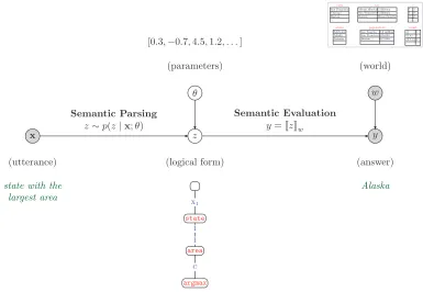
Our statistical methodology consists of two steps: (i) semantic parsing (p(z|x;θ)): an utterancex
is mapped to a logical formzby drawing from a log-linear distribution parametrized by a vectorθ; and (ii) evaluation ([[z]]w): the logical formzis evaluated with respect to the worldw
(database of facts) to deterministically produce an answery. The figure also shows an example configuration of the variables around the graphical model. Logical formszare represented as labeled trees. During learning, we are givenwand (x,y) pairs (shaded nodes) and try to infer the latent logical formszand parametersθ.
2010; Artzi and Zettlemoyer 2011; Goldwasser et al. 2011; Liang, Jordan, and Klein 2011). It is in this vein that we develop our present work. Specifically, given a set of (x,y) example pairs, wherex is an utterance (e.g., a question) and y is the corresponding answer, we wish to learn a mapping fromxtoy. What makes this mapping particularly interesting is that it passes through a latent logical formz, which is necessary to capture the semantic complexities of natural language. Also note that whereas the logical form zwas the end goal in much of earlier work on semantic parsing, for us it is just an intermediate variable—a means towards an end. Figure 2 shows the graphical model which captures the learning setting we just described: The questionx, answery, and world/database w are all observed. We want to infer the logical forms z and the parametersθof the semantic parser, which are unknown quantities.
Computational Linguistics Volume 39, Number 2
should the formal language for the logical formszbe, and (ii) what are the compositional mechanisms for constructing those logical forms?
The semantic parsing literature has considered many different formal languages for representing logical forms, including SQL (Giordani and Moschitti 2009), Prolog (Zelle and Mooney 1996; Tang and Mooney 2001), a simple functional query language called FunQL (Kate, Wong, and Mooney 2005), and lambda calculus (Zettlemoyer and Collins 2005), just to name a few. The construction mechanisms are equally diverse, in-cluding synchronous grammars (Wong and Mooney 2007), hybrid trees (Lu et al. 2008), Combinatory Categorial Grammars (CCG) (Zettlemoyer and Collins 2005), and shift-reduce derivations (Zelle and Mooney 1996). It is worth pointing out that the choice of formal language and the construction mechanism are decisions which are really more orthogonal than is often assumed—the former is concerned with what the logical forms look like; the latter, with how to generate a set of possible logical forms compositionally given an utterance. (Howto score these logical forms is yet another dimension.)
Existing systems are rarely based on the joint design of the formal language and the construction mechanism; one or the other is often chosen for convenience from existing implementations. For example, Prolog and SQL have often been chosen as formal languages for convenience in end applications, but they were not designed for representing the semantics of natural language, and, as a result, the construction mechanism that bridges the gap between natural language and formal language is generally complex and difficult to learn. CCG (Steedman 2000) is quite popular in computational linguistics (for example, see Bos et al. [2004] and Zettlemoyer and Collins [2005]). In CCG, logical forms are constructed compositionally using a small handful of combinators (function application, function composition, and type raising). For a wide range of canonical examples, CCG produces elegant, streamlined analyses, but its success really depends on having a good, clean lexicon. During learning, there is often a great amount of uncertainty over the lexical entries, which makes CCG more cumbersome. Furthermore, in real-world applications, we would like to handle disflu-ent utterances, and this further strains CCG by demanding either extra type-raising rules and disharmonic combinators (Zettlemoyer and Collins 2007) or a proliferation of redundant lexical entries for each word (Kwiatkowski et al. 2010).
To cope with the challenging demands of program induction, we break away from tradition in favor of a new formal language and construction mechanism, which we call
dependency-based compositional semantics(DCS). The guiding principle behind DCS is to provide a simple and intuitive framework for constructing and representing logical forms. Logical forms in DCS are tree structures calledDCS trees. The motivation is two-fold: (i) DCS trees are meant to parallel syntactic dependency trees, which facilitates parsing; and (ii) a DCS tree essentially encodes a constraint satisfaction problem, which can be solved efficiently using dynamic programming to obtain the denotation of a DCS tree. In addition, DCS provides amark–executeconstruct, which provides a uniform way of dealing with scope variation, a major source of trouble in any semantic for-malism. The construction mechanism in DCS is a generalization of labeled dependency parsing, which leads to simple and natural algorithms. To a linguist, DCS might appear unorthodox, but it is important to keep in mind that our primary goal is effective program induction, not necessarily to model newlinguistic phenomena in the tradition of formal semantics.
work that also learns from answers instead of logical forms (Clarke et al. 2010). What is perhaps a more significant result is that our system obtains comparable accuracies to state-of-the-art systems that do rely on annotated logical forms. This demonstrates the viability of training accurate systems with much less supervision than before.
The rest of this article is organized as follows: Section 2 introduces DCS, our new semantic formalism. Section 3 presents our probabilistic model and learning algorithm. Section 4 provides an empirical evaluation of our methods. Section 5 situates this work in a broader context, and Section 6 concludes.
2. Representation
In this section, we present the main conceptual contribution of this work, dependency-based compositional semantics (DCS), using the U.S. geography domain (Zelle and Mooney 1996) as a running example. To do this, we need to define the syntax and semantics of the formal language. The syntax is defined in Section 2.2 and is quite straightforward: The logical forms in the formal language are simply trees, which we callDCS trees. In Section 2.3, we give a type-theoretic definition ofworlds(also known as databases or models) with respect to which we can define the semantics of DCS trees. The semantics, which is the heart of this article, contains two main ideas: (i) using trees to represent logical forms as constraint satisfaction problems or extensions thereof, and (ii) dealing with cases when syntactic and semantic scope diverge (e.g., for general-ized quantification and superlative constructions) using a new construct which we call
mark–execute. We start in Section 2.4 by introducing the semantics of a basic version of DCS which focuses only on (i) and then extend it to the full version (Section 2.5) to account for (ii).
Finally, having fully specified the formal language, we describe a construction mechanism for mapping a natural language utterance to a set of candidate DCS trees (Section 2.6).
2.1 Notation
Operations on tuples will play a prominent role in this article. For a sequence1 v=
(v1,. . .,vk), we use |v|=kto denote the length of the sequence. For two sequencesu andv, w e useu+v=(u1,. . .,u|u|,v1,. . .,v|v|) to denote their concatenation.
1 We use the termsequenceto refer to both tuples (v1,. . .,vk) and arrays [v1,. . .,vk]. For our purposes, there
Computational Linguistics Volume 39, Number 2
For a sequence of positive indicesi=(i1,. . .,im), letvi=(vi1,. . .,vim) consist of the
components ofv specified byi; we callvi the projection of vontoi. We use negative indices to exclude components: v−i =(v(1,...,|v|)\i). We can also combine sequences of indices by concatenation: vi,j =vi+vj. Some examples: if v=(a,b,c,d), then v2 =b, v3,1=(c,a),v−3 =(a,b,d),v3,−3 =(c,a,b,d).
2.2 Syntax of DCS Trees
The syntax of the DCS formal language is built from two ingredients, predicates and relations:
r
LetP be a set ofpredicates. We assume thatP contains a special null predicate ø, domain-independent predicates (e.g.,count,<,>, and=), and domain-specific predicates (for the U.S. geography domain,state,river, border, etc.). Right now, think of predicates as just labels, w hich have yet to receive formal semantics.r
LetRbe the set ofrelations. Note that unlike the predicatesP, which canvary across domains, the relationsRare fixed. The full set of relations are shown in Table 1. For now, just think of relations as labels—their semantics will be defined in Section 2.4.
The logical forms in DCS are called DCS trees. A DCS tree is a directed rooted tree in which nodes are labeled with predicates and edges are labeled with relations; each node also maintains an ordering over its children. Formally:
Definition 1 (DCS trees)
LetZbe the set of DCS trees, where eachz∈Zconsists of (i) a predicatez.p∈Pand (ii) a sequence of edgesz.e=(z.e1,. . .,z.em). Each edgeeconsists of a relatione.r∈R(see
Table 1) and a child treee.c∈Z.
We will either draw a DCS tree graphically or write it compactly asp;r1:c1;. . .;rm:cm
wherepis the predicate at the root node andc1,. . .,cm are itsmchildren connected via edges labeled with relationsr1,. . .,rm, respectively. Figure 3(a) shows an example of a DCS tree expressed using both graphical and compact formats.
Table 1
Possible relations that appear on edges of DCS trees. Basic DCS uses only the join and aggregate relations; the full version of DCS uses all of them.
RelationsR
Name Relation Description of semantic function
join jjforj,j∈ {1, 2,. . .} j-th component of parent=j-th component of child
aggregate Σ parent=set of feasible values of child
extract E mark node for extraction
quantify Q mark node for quantification, negation
compare C mark node for superlatives, comparatives
Figure 3
(a) An example of a DCS tree (written in both the mathematical and graphical notations). Each node is labeled with a predicate, and each edge is labeled with a relation. (b) A DCS treezwith only join relations encodes a constraint satisfaction problem, represented here as a lambda calculus formula. For example, the root node labelcitycorresponds to a unary predicate city(c), the right child node labelloccorresponds to a binary predicateloc() (w hereis a pair), and the edge between them denotes the constraintc1=1(where the indices correspond to the two labels on the edge). (c) The denotation ofzis the set of feasible values for the root node.
A DCS tree is a logical form, but it is designed to look like a syntactic dependency tree, only with predicates in place of words. As we’ll see over the course of this section, it is this transparency between syntax and semantics provided by DCS which leads to a simple and streamlined compositional semantics suitable for program induction.
2.3 Worlds
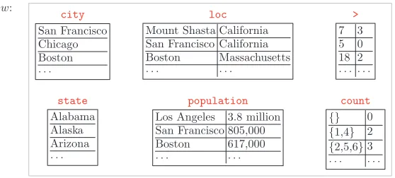
[image:7.486.54.333.468.594.2]In the context of question answering, the DCS tree is a formal specification of the question. To obtain an answer, we still need to evaluate the DCS tree with respect to a database of facts (see Figure 4 for an example). We will use the termworldto refer
Figure 4
Computational Linguistics Volume 39, Number 2
to this database (it is sometimes also called a model, but we avoid this term to avoid confusion with the probabilistic model for learning that we will present in Section 3.1). Throughout this work, we assume the world is fully observed and fixed, which is a realistic assumption for building natural language interfaces to existing databases, but questionable for modeling the semantics of language in general.
2.3.1 Types and Values. To define a world, we start by constructing a set of valuesV. The exact set of values depends on the domain (we will continue to use U.S. geog-raphy as a running example). Briefly, V contains numbers (e.g., 3∈V), strings (e.g., Washington∈ V), tuples (e.g., (3,Washington)∈ V), sets (e.g.,{3,Washington} ∈V), and other higher-order entities.
To be more precise, we constructVrecursively. First, define a set of primitive values V, which includes the following:
r
Numeric values. Each value has the formx:t∈V, wherex∈Ris a real number andt∈ {number,ordinal,percent,length,. . .}is a tag. The tag allows us to differentiate 3, 3rd, 3%, and 3 miles—this will be important in Section 2.6.3. We simply writexfor the valuex:number.r
Symbolic values. Each value has the formx:t∈V, wherexis a string (e.g., Washington) andt∈ {string,city,state,river,. . .}is a tag. Again, the tag allows us to differentiate, for example, the entitiesWashington:city andWashington:state.Now we build the full set of valuesV from the primitive valuesV. To defineV, w e need a bit more machinery: To avoid logical paradoxes, we construct V in increasing order of complexity using types (see Carpenter [1998] for a similar construction). The casual reader can skip this construction without losing any intuition.
Define the set of typesT to be the smallest set that satisfies the following properties:
1. The primitive type∈T;
2. The tuple type (t1,. . .,tk)∈T for eachk≥0 and each non-tuple type
ti∈T fori=1,. . .,k; and
3. The set type{t} ∈T for each tuple typet∈T.
Note that{},{{}}, and (()) are not valid types.
For each typet∈T, we construct a corresponding set of valuesVt:
1. For the primitive typet=, the primitive valuesVhave already been specified. Note that these types are rather coarse: Primitive values with different tags are considered to have the same type.
2. For a tuple typet=(t1,. . .,tk),Vtis the cross product of the values of its
component types:
LetV=∪t∈TVtbe the set of all possible values.
A world maps each predicate to itssemantics, which is a set of tuples (see Figure 4 for an example). First, letTTUPLE ⊂T be the tuple types, which are the ones of the form (t1,. . .,tk) for somek. LetV{TUPLE}denote all the sets of tuples (with the same type):
V{TUPLE} def
=
t∈TTUPLE
V{t} (3)
Now we define a world formally.
Definition 2 (World)
A w orld w:P →V{TUPLE}∪ {V} is a function that maps each non-null predicate p∈
P\{ø}to a set of tuplesw(p)∈V{TUPLE}and maps the null predicate ø to the set of all values (w(ø)=V).
For a set of tuplesAwith the same arity, let ARITY(A)=|x|, wherex∈Ais arbitrary; if Ais empty, then ARITY(A) is undefined. Nowfor a predicatep∈P and worldw, define ARITYw(p), the arity of predicatepwith respect tow, as follows:
ARITYw(p)=
1 ifp=ø
ARITY(w(p)) ifp=ø (4)
The null predicate has arity 1 by fiat; the arity of a non-null predicatepis inherited from the tuples inw(p).
Remarks.In higher-order logic and lambda calculus, we construct function types and values, whereas in DCS, we construct tuple types and values. The two are equivalent in representational power, but this discrepancy does point out the fact that lambda calculus is based on function application, whereas DCS, as we will see, is based on declarative constraints. The set type{(,)}in DCS corresponds to the function type
→(→bool). In DCS, there is no explicitbooltype—it is implicitly represented by using sets.
Computational Linguistics Volume 39, Number 2
predicate that maps to the set of U.S. states (state), another predicate that maps to the set of pairs of entities and where they are located (loc), and so on:
w(state)={(California:state), (Oregon:state),. . .} (5) w(loc)={(San Francisco:city,California:state),. . .} (6)
. . . (7)
To shorten notation, we use state abbreviations (e.g.,CA=California:state).
The worldwalso specifies the semantics of several domain-independent predicates (think of these as helper functions), which usually correspond to an infinite set of tuples. Functions are represented in DCS by a set of input–output pairs. For example, the semantics of thecounttpredicate (for each typet∈T) contains pairs of setsSand their cardinalities|S|:
w(countt)={(S,|S|) :S∈V{(t)}} ∈V{({(t)},)} (8)
As another example, consider the predicateaveraget(for eacht∈T), which takes a set of key–value pairs (with keys of typet) and returns the average value. For notational convenience, we treat an arbitrary set of pairsSas a set-valued function: We letS1={x: (x,y)∈S}denote the domain of the function, and abusing notation slightly, we define the functionS(x)={y: (x,y)∈S}to be the set of valuesythat co-occur with the given x. The semantics ofaveragetcontains pairs of sets and their averages:
w(averaget)=
(S,z) :S∈V{(t,)},z=|S1|−1
x∈S1
|S(x)|−1
y∈S(x) y
∈V{({(t,)},)}
(9)
Similarly, we can define the semantics ofargmintandargmaxt, which each takes a set of key–value pairs and returns the keys that attain the smallest (largest) value:
w(argmint)=
(S,z) :S∈V{(t,)},z∈argmin
x∈S1
minS(x)
∈V{({(t,)},t)} (10)
w(argmaxt)=
(S,z) :S∈V{(t,)},z∈argmax
x∈S1
maxS(x)
∈V{({(t,)},t)} (11)
The extra min and max is needed becauseS(x) could contain more than one value. We also impose thatw(argmint) contains only (S,z) such thatyis numeric for all (x,y)∈S; thusargmintdenotes a partial function (same forargmaxt).
2.4.1 Basic DCS Trees as Constraint Satisfaction Problems.Letzbe a DCS tree with only join relations on its edges. In this case,zencodes a CSP as follows: For each nodexinz, the CSP has a variable with valuea(x); the collection of these values is referred to as an assignment a. The predicates and relations ofzintroduce constraints:
1. a(x)∈w(p) for each nodexlabeled with predicatep∈P; and
2. a(x)j=a(y)jfor each edge (x,y) labeled with j
j∈R, which says that the
j-th component ofa(x) must equal thej-th component ofa(y).
We say that an assignmentaisfeasibleif it satisfies these two constraints. Next, for a node x, defineV(x)={a(x) : assignmentais feasible}as the set of feasible values forx—these are the ones that are consistent with at least one feasible assignment. Finally, we define the denotation of the DCS treezwith respect to the worldwto bezw=V(x0), where x0is the root node ofz.
Figure 3(a) shows an example of a DCS tree. The corresponding CSP has four vari-ablesc,m,,s.2In Figure 3(b), we have written the equivalent lambda calculus formula. The non-root nodes are existentially quantified, the root nodec is λ-abstracted, and all constraints introduced by predicates and relations are conjoined. Theλ-abstraction ofcrepresents the fact that the denotation is the set of feasible values forc (note the equivalence between the Boolean functionλc.p(c) and the set{c:p(c)}).
Remarks. Note that CSPs only allowexistential quantification and conjunction. Why did we choose this particular logical subset as a starting point, rather than allowing universal quantification, negation, or disjunction? There seems to be something fun-damental about this subset, which also appears in Discourse Representation Theory (DRT) (Kamp and Reyle 1993; Kamp, van Genabith, and Reyle 2005). Briefly, logical forms in DRT are called Discourse Representation Structures (DRSs), each of which contains (i) a set of existentially quantified discourse referents (variables), (ii) a set of conjoined discourse conditions (constraints), and (iii) nested DRSs. If we exclude nested DRSs, a DRS is exactly a CSP.3The default existential quantification and conjunction are quite natural for modeling cross-sentential anaphora: Newvariables can be added to
2 Technically, the node iscand the variable isa(c), but we usecto denote the variable to simplify notation. 3 Unlike the CSPs corresponding to DCS trees, the CSPs corresponding to DRSs need not be
Computational Linguistics Volume 39, Number 2
a DRS and connected to other variables. Indeed, DRT was originally motivated by these phenomena (see Kamp and Reyle [1993] for more details).4
Tree-structured CSPs can capture unboundedly complex recursive structures—such as cities in states that border states that have rivers that. . .. Trees are limited, however, in that they are unable to capture long-distance dependencies such as those arising from anaphora. For example, in the phrasea state with a river that traverses its capital,itsbinds to state, but this dependence cannot be captured in a tree structure. A solution is to simply add an edge between the its node and the state node that forces the two nodes to have the same value. The result is still a well-defined CSP, though not a tree-structured one. The situation would become trickier if we were to integrate the other relations (aggregate, mark, and execute). We might be able to incorporate some ideas from Hybrid Logic Dependency Semantics (Baldridge and Kruijff 2002; White 2006), given that hybrid logic extends the tree structures of modal logic withnominals, thereby allowing a node to freely reference other nodes. In this article, however, we will stick to trees and leave the full exploration of non-trees for future work.
2.4.2 Computation of Join Relations.So far, we have given a declarative definition of the denotation zw of a DCS treezwith only join relations. Now we will show how to computezwefficiently. Recall that the denotation is the set of feasible values for the root node. In general, finding the solution to a CSP is NP-hard, but for trees, we can exploit dynamic programming (Dechter 2003). The key is that the denotation of a tree depends on its subtrees only through their denotations:
p;jj1 1:
c1;· · ·;jm jm:cm
w
=w(p) ∩
m
i=1 {v:vj
i=tji,t∈ciw} (12)
On the right-hand side of Equation (12), the first termw(p) is the set of values that satisfy the node constraint, and the second term consists of an intersection across allmedges of{v:vji =tji,t∈ciw}, which is the set of valuesvwhich satisfy the edge constraint
with respect to some valuetfor the childci.
To further flesh out this computation, we express Equation (12) in terms of two operations:joinandproject. Join takes a cross product of two sets of tuples and retains the resulting tuples that match the join constraint:
Aj,jB={u+v:u∈A,v∈B,uj=vj} (13)
Project takes a set of tuples and retains a fixed subset of the components:
A[i]={vi:v∈A} (14)
The denotation in Equation (12) can nowbe expressed in terms of these join and project operations:
p;j1
j1:c1;· · ·;
jm jm:cm
w
=((w(p)j
1,j1c1w)[i]· · ·jm,jm cmw)[i] (15)
2.4.3 Aggregate Relation. Thus far, we have focused on DCS trees that only use join relations, which are insufficient for capturing higher-order phenomena in language. For example, consider the phrasenumber of major cities. Suppose thatnumbercorresponds to thecountpredicate, and thatmajor citiesmaps to the DCS treecity;1
1:major . We cannot simply joincountwith the root of this DCS tree becausecountneeds to be joined with thesetof major cities (the denotation ofcity;1
1:major ), not just a single city. We therefore introduce the aggregate relation (Σ) that takes a DCS subtree and reifies its denotation so that it can be accessed by other nodes in its entirety. Consider a treeø;Σ:c , where the root is connected to a childcviaΣ. The denotation of the root is simply the singleton set containing the denotation ofc:
ø;Σ:c w={(cw)} (16)
Figure 5(a) shows the DCS tree for our running example. The denotation of the middle node is {(s)}, where s is all major cities. Everything above this node is an ordinary CSP:sconstrains thecountnode, which in turns constrains the root node to |s|. Figure 5(b) shows another example of using the aggregate relationΣ. Here, the node right aboveΣis constrained to be a set of pairs of major cities and their populations. Theaveragepredicate then computes the desired answer.
To represent logical disjunction in natural language, we use the aggregate relation and two predicates,unionandcontains, which are defined in the expected way:
w(union)={(A,B,C) :C=A∪B,A∈V{},B∈V{}} (17)
w(contains)={(A,x) :x∈A,A∈V{}} (18)
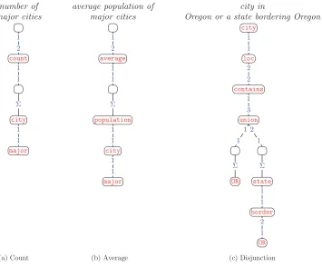
whereA,B,C∈V{}are sets of primitive values (see Section 2.3.1). Figure 5(c) shows an example of a disjunctive construction: We use the aggregate relations to construct two sets, one containing Oregon, and the other containing states bordering Oregon. We take the union of these two sets;containstakes the set and reads out an element, which then constrains thecitynode.
Remarks.A DCS tree that contains only join and aggregate relations can be viewed as a collection of tree-structured CSPs connected via aggregate relations. The tree struc-ture still enables us to compute denotations efficiently based on the recurrences in Equations (15) and (16).
Computational Linguistics Volume 39, Number 2
Figure 5
Examples of DCS trees that use the aggregate relation (Σ) to (a) compute the cardinality of a set, (b) take the average over a set, (c) represent a disjunction over two conditions. The aggregate relation sets the parent node deterministically to the denotation of the child node. Nodes with the special null predicate ø are represented as empty nodes.
making nested DRSs. It turns out that the abstraction operator is sufficient to obtain the full representational power of DRT, and subsumes generalized quantification and disjunction constructs in DRT. By analogy, we use the aggregate relation to handle disjunction (Figure 5(c)) and generalized quantification (Section 2.5.6).
DCS restricted to join relations is less expressive than first-order logic because it does not have universal quantification, negation, and disjunction. The aggregate rela-tion is analogous to lambda abstracrela-tion, and in basic DCS we use the aggregate relarela-tion to implement those basic constructs using higher-order predicates such asnot,every, and union. We can also express logical statements such as generalized quantification, which go beyond first-order logic.
2.5 Semantics of DCS Trees with Mark–Execute (Full Version)
Basic DCS includes two types of relations, join and aggregate, but it is already quite expressive. In general, however, it is not enough just to be able to express the meaning of a sentence using some logical form; we must be able to derive the logical form compositionally and simply from the sentence.
Figure 6
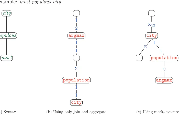
Two semantically equivalent DCS trees are shown in (b) and (c). The DCS tree in (b), which uses the join and aggregate relations in the basic DCS, does not align well with the syntactic structure ofmost populous city(a), and thus is undesirable. The DCS tree in (c), by using the mark–execute construct, aligns much better, withcityrightfully dominating its modifiers. The full version of DCS allows us to construct (c), which is preferable to (b).
already use a DCS tree with only join and aggregate relations to express the correct semantics of the superlative construction. Note, however, that the two structures are quite divergent—the syntactic head iscityand the semantic head isargmax. This diver-gence runs counter to a principal desideratum of DCS, which is to create a transparent interface between coarse syntax and semantics.
In this section, we introduce mark and execute relations, which will allow us to use the DCS tree in Figure 6(c) to represent the semantics associated with Figure 6(a); these two are more similar than (a) and (b). The focus of this section is on this mark– execute construct—using mark and execute relations to give proper semantically scoped denotations to syntactically scoped tree structures.
The basic intuition of the mark–execute construct is as follows: We mark a node lowin the tree with amark relation; then, higher up in the tree, we invoke it with a correspondingexecute relation(Figure 7). For our example in Figure 6(c), we mark the populationnode, which puts the childargmaxin a temporary store; when we execute thecitynode, we fetch the superlative predicateargmaxfrom the store and invoke it.
This divergence between syntactic and semantic scope arises in other linguistic contexts besides superlatives, such as quantification and negation. In each of these cases, the general template is the same: A syntactic modifier lowin the tree needs to have semantic force higher in the tree. A particularly compelling case of this divergence happens with quantifier scope ambiguity (e.g.,Some river traverses every city5), where the
Computational Linguistics Volume 39, Number 2
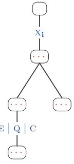
Figure 7
The template for the mark–execute construct. A mark relation (one ofE,Q,C) “stores” the modifier. Then an execute relation (of the formXifor indicesi) higher up “recalls” the modifier and applies it at the desired semantic point.
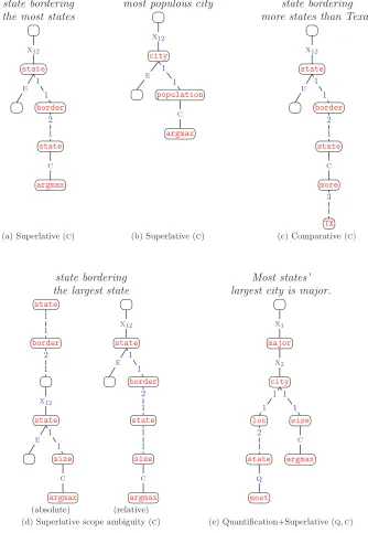
quantifiers appear in fixed syntactic positions, but the surface and inverse scope read-ings correspond to different semantically scoped denotations. Analogously, a single syn-tactic structure involving superlatives can also yield two different semantically scoped denotations—the absolute and relative readings (e.g., state bordering the largest state6). The mark–execute construct provides a unified framework for dealing all these forms of divergence between syntactic and semantic scope. See Figures 8 and 9 for concrete examples of this construct.
2.5.1 Denotations.We nowformalize the mark–execute construct. We sawthat the mark– execute construct appears to act non-locally, putting things in a store and retrieving them later. This means that if we want the denotation of a DCS tree to only depend on the denotations of its subtrees, the denotations need to contain more than the set of feasible values for the root node, as was the case for basic DCS. We need to augment de-notations to include information about all marked nodes, because these can be accessed by an execute relation higher up in the tree.
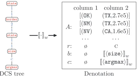
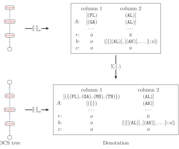
More specifically, letzbe a DCS tree andd=zwbe its denotation. The denotation d consists ofn columns. The first column always corresponds to the root node of z, and the rest of the columns correspond to non-root marked nodes inz. In the example in Figure 10, there are two columns, one for the rootstatenode and the other forsize node, which is marked byC. The columns are ordered according to a pre-order traversal ofz, so column 1 always corresponds to the root node. The denotationdcontains a set of arraysd.A, where each array represents a feasible assignment of values to the columns ofd; note that we quantify over non-marked nodes, so they do not correspond to any column in the denotation. For example, in Figure 10, the first array ind.Acorresponds to assigning (OK) to thestatenode (column 1) and (TX, 2.7e5) to thesizenode (column 2). If there are no marked nodes,d.Ais basically a set of tuples, which corresponds to a denotation in basic DCS. For each marked node, the denotationdalso maintains astore
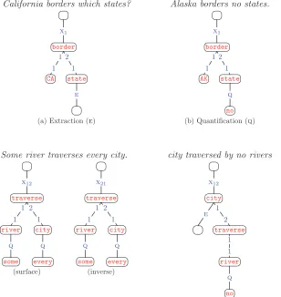
Figure 8
Examples of DCS trees that use the mark–execute construct with theEandQmark relations. (a) The head verbborders, which needs to be returned, has a direct objectstatesmodified by
which. (b) The quantifiernois syntactically dominated bystatebut needs to take wider scope. (c) Two quantifiers yield two possible readings; we build the same basic structure, marking both quantifiers; the choice of execute relation (X12versusX21) determines the reading. (d) We use two mark relations,Qonriverfor the negation, andEoncityto force the quantifier to be computed for each value ofcity.
with information to be retrieved when that marked node is executed. A storeσfor a marked node contains the following: (i) the mark relationσ.r(Cin the example), (ii) the base denotationσ.b, which essentially corresponds to denotation of the subtree rooted at the marked node excluding the mark relation and its subtree (size win the example), and (iii) the denotation of the child of the mark relation (argmax win the example). The store of any unmarked nodes is always empty (σ=ø).
Definition 3 (Denotations)
LetDbe the set ofdenotations, where each denotationd∈Dconsists of
r
a set of arraysd.A, where each arraya=[a1,. . .,an]∈d.Ais a sequence ofComputational Linguistics Volume 39, Number 2
Figure 9
Figure 10
Example of the denotation for a DCS tree (with the compare relationC). This denotation has two columns, one for each active node—the root nodestateand the marked nodesize.
r
a sequence ofn stores d.σ=(d.σ1,. . .,d.σn), where each storeσcontains amark relationσ.r∈ {E,Q,C, ø}, a base denotationσ.b∈D∪ {ø}, and a child denotationσ.c∈D∪ {ø}.
Note that denotations are formally defined without reference to DCS trees (just as sets of tuples were in basic DCS), but it is sometimes useful to refer to the DCS tree that generates that denotation.
For notational convenience, we write d as A; (r1,b1,c1);. . .; (rn,bn,cn) . Also let d.ri=d.σi.r, d.bi=d.σi.b, and d.ci=d.σi.c. Let d{σi=x} be the denotation which is identical to d, except with d.σi=x; d{ri=x}, d{bi=x}, and d{ci=x} are defined
analogously. We also define a project operation for denotations:A;σ [i]def= {ai :a∈ A};σi . Extending this notation further, we use ø to denote the indices of thenon-initial columns with empty stores(i>1 such thatd.σi=ø). We can then used[−ø] to represent
projecting away the non-initial columns with empty stores. For the denotation d in Figure 10,d[1] keeps column 1,d[−ø] keeps both columns, andd[2,−2] swaps the two columns.
In basic DCS, denotations are sets of tuples, which works quite well for repre-senting the semantics ofwh-questions such asWhat states border Texas?But what about polar questions such asDoes Louisiana border Texas?The denotation should be a simple Boolean value, which basic DCS does not represent explicitly. Using our new deno-tations, we can represent Boolean values explicitly using zero-column structures:true
corresponds to a singleton set containing just the empty array (dT ={[ ]} ) andfalse is the empty set (dF=∅ ).
Having described denotations as n-column structures, we now give the formal mapping from DCS trees to these structures. As in basic DCS, this mapping is defined recursively over the structure of the tree. We have a recurrence for each case (the first line is the base case, and each of the others handles a different edge relation):
p w={[v] :v∈w(p)}; ø [base case] (19)
p;e;jj:c
w
=p;e w−j,jøcw [join] (20)
Computational Linguistics Volume 39, Number 2
p;e;Xi:c w=p;e w −ø
∗,∗xi(cw) [execute] (22)
p;e;E:c w=M(p;e w,E,cw) [extract] (23) p;e;C:c w=M(p;e w,C,cw) [compare] (24) p;Q:c;e w=M(p;e w,Q,cw) [quantify] (25)
We define the operations−ø
j,j,Σ,Xi, andMin the remainder of this section.
2.5.2 Base Case.Equation (19) defines the denotation for a DCS treezwith a single node with predicate p. The denotation ofzhas one column whose arrays correspond to the tuplesw(p); the store for that column is empty.
2.5.3 Join Relations. Equation (20) defines the recurrence for join relations. On the left-hand side,
p;e;jj:c
is a DCS tree withpat the root, a sequence of edgesefollowed by a final edge w ith relationjjconnected to a child DCS treec. On the right-hand side, we take the recursively computed denotation ofp;e , the DCS tree without the final edge, and perform ajoin-project-inactiveoperation (notated−ø
j,j) with the denotation of the
child DCS treec.
The join-project-inactive operation joins the arrays of the two denotations (this is the core of the join operation in basic DCS—see Equation (13)), and then projects away the non-initial empty columns:7
A;σ −j,jø A;σ =A;σ+σ [−ø], where (26)
A={a+a:a∈A,a∈A,a1j=a1j}
We concatenate all arrays a∈Awith all arrays a∈A that satisfy the join condition a1j=a1j. The sequences of stores are simply concatenated: (σ+σ
). Finally, any
non-initial columns with empty stores are projected away by applying·[−ø].
Note that the join works on column 1; the other columns are carried along for the ride. As another piece of convenient notation, we use∗to represent all components, so
−∗,ø∗imposes the join condition that the entire tuple has to agree (a1 =a1).
2.5.4 Aggregate Relations. Equation (21) defines the recurrence for aggregate relations. Recall that in basic DCS, aggregate (16) simply takes the denotation (a set of tuples) and puts it into a set. Now, the denotation is not just a set, so w e need to generalize this operation. Specifically, the aggregate operation applied to a denotation forms a set out of the tuples in the first column for each setting of the rest of the columns:
Σ(A;σ )=A∪A;σ (27) A={[S(a),a2,. . .,an] :a∈A}
S(a)={a1: [a1,a2,. . .,an]∈A}
A ={[∅,a2,. . .,an] :∀i∈ {2,. . .,n}, [ai]∈σi.b.A[1],¬∃a1,a∈A}
stores. In particular, for each columni∈ {2,. . .,n}, we have conveniently stored a base denotationσi.b. We consider anyai that occurs in column 1 of the arrays of this base
denotation ([ai]∈σi.b.A[1]). For thisa2,. . .,an, w e include [∅,a2,. . .,an] inAas long as
a2,. . .,andoes not co-occur with anya1. An example is given in Figure 11.
[image:21.486.56.413.314.611.2]The reason for storing base denotations is thus partially revealed: The arrays rep-resent feasible values of a CSP and can only contain positive information. When we aggregate, we need to access possibly empty sets of feasible values—a kind of negative information, which can only be recovered from the base denotations.
Figure 11
Computational Linguistics Volume 39, Number 2
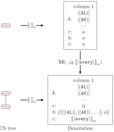
2.5.5 Mark Relations. Equations (23), (24), and (25) each processes a different mark relation. We define a general mark operation, M(d,r,c) which takes a denotationd, a mark relationr∈ {E,Q,C}and a child denotationc, and sets the store ofdin column 1 to be (r,d,c):
M(d,r,c)=d{r1=r,b1 =d,c1 =c} (28)
The base denotation of the first columnb1 is set to the current denotationd. This, in some sense, creates a snapshot of the current denotation. Figure 12 shows an example of the mark operation.
2.5.6 Execute Relations.Equation (22) defines the denotation of a DCS tree where the last edge of the root is an execute relation. Similar to the aggregate case (21), we recurse on the DCS tree without the last edge (p;e ) and then join it to the result of applying the execute operationXito the denotation of the child (cw).
[image:22.486.59.291.359.627.2]The execute operation Xi is the most intricate part of DCS and is what does the heavy lifting. The operation is parametrized by a sequence of distinct indices i that specifies the order in which the columns should be processed. Specifically,iindexes into the subsequence of columns with non-empty stores. We then process this subsequence of columns in reverse order, where processing a column means performing some op-erations depending on the stored relation in that column. For example, suppose that columns 2 and 3 are the only non-empty columns. ThenX12processes column 3 before column 2. On the other hand,X21processes column 2 before column 3. We first define
Figure 12
Figure 13
An example of applying the execute operation on column 1 with the extract relationE. The denotation prior to execution consists of two columns: column 1 corresponds to theborder node; column 2 to thestatenode. The join relations and predicatesCAandstateconstrain the arraysAin the denotation to include only the states that border California. After execution, the non-marked column 1 is projected away, leaving only thestatecolumn with its store emptied.
the execute operationXifor a single columni. There are three distinct cases, depending
on the relation stored in columni:
Extraction.For a denotation dwith the extract relation E in column i, executingXi(d)
involves three steps: (i) moving columni to before column 1 (·[i,−i]), (ii) projecting away non-initial empty columns (·[−ø]), and (iii) removing the store (·{σ1=ø}):
Xi(d)=d[i,−i][−ø]{σ1 =ø} ifd.ri=E (29)
An example is given in Figure 13. There are two main uses of extraction.
1. By default, the denotation of a DCS tree is the set of feasible values of the root node (which occupies column 1). To return the set of feasible values of another node, we mark that node withE. Upon execution, the feasible values of that node move into column 1. Extraction can be used to handle in situ questions (see Figure 8(a)).
Computational Linguistics Volume 39, Number 2
markingx(withE) and executingybeforex(see Figure 8(d,e) for examples). The extract relationE(in fact, any mark relation) signifies that we want to control the scope of a node, and the execute relation allows us to set that scope.
Generalized Quantification.Generalized quantifiers are predicates on two sets, arestrictor Aand anuclear scopeB. For example,
w(some)={(A,B) :A∩B>0} (30) w(every)={(A,B) :A⊂B} (31)
w(no)={(A,B) :A∩B=∅} (32)
w(most)={(A,B) :|A∩B|> 1
2|A|} (33)
We think of the quantifier as a modifier which always appears as the child of aQrelation; the restrictor is the parent. For example, in Figure 8(b),nocorresponds to the quantifier andstatecorresponds to the restrictor. The nuclear scope should be the set of all states that Alaska borders. More generally, the nuclear scope is the set of feasible values of the restrictor node with respect to the CSP that includes all nodes between the mark and execute relations. The restrictor is also the set of feasible values of the restrictor node, but with respect to the CSP corresponding to the subtree rooted at that node.8
We implement generalized quantifiers as follows: Letdbe a denotation and suppose we are executing column i. We first construct a denotation for the restrictordAand a denotation for the nuclear scopedB. For the restrictor, we take the base denotation in columni(d.bi)—remember that the base denotation represents a snapshot of the restric-tor node before the nuclear scope constraints are added. For the nuclear scope, we take the complete denotation d (which includes the nuclear scope constraints) and extract columni(d[i,−i][−ø]{σ1=ø}—see (29)). We then constructdAanddBby applying the
aggregate operation to each. Finally, we join these sets with the quantifier denotation, stored ind.ci:
xi(d)=
d.ci−1,1ødA
−2,1ødB
[−1] ifd.ri=Q, where (34)
dA= Σ(d.bi) (35)
dB= Σ(d[i,−i][−ø]{σ1=ø}) (36)
When there is one quantifier, think of the execute relation as performing a syntactic rewriting operation, as shown in Figure 14(b). For more complex cases, we must defer to (34).
Figure 8(c) shows an example with two interacting quantifiers. The denotation of the DCS tree before execution is the same in both readings, as shown in Figure 15. The
Figure 14
(a) An example of applying the execute operation on columniwith the quantify relationQ. Before executing, note thatA={}(because Alaska does not border any states). The restrictor (A) is the set of all states, and the nuclear scope (B) is empty. Because the pair (A,B) does exist in
w(no), the final denotation is{[ ]} (which represents true). (b) Although the execute operation actually works on the denotation, think of it in terms of expanding the DCS tree. We introduce an extra projection relation [−1], which projects away the first column of the child subtree’s denotation.
quantifier scope ambiguity is resolved by the choice of execute relation:X12gives the surface scope reading,X21gives the inverse scope reading.
Figure 8(d) shows how extraction and quantification work together. First, theno quantifier is processed for eachcity, which is an unprocessed marked node. Here, the extract relation is a technical trick to givecitywider scope.
[image:25.486.56.414.518.639.2]Comparatives and Superlatives.Comparative and superlative constructions involve com-paring entities, and for this we rely on a setSof entity–degree pairs (x,y), wherexis an
Figure 15
Computational Linguistics Volume 39, Number 2
entity andyis a numeric degree. Recall that we can treatSas a function, which maps an entityx to the set of degreesS(x) associated with x. Note that this set can contain multiple degrees. For example, in the relative reading ofstate bordering the largest state, we would have a degree for the size of each neighboring state.
Superlatives use theargmaxandargminpredicates, which are defined in Section 2.3. Comparatives use themoreandlesspredicates:w(more) contains triples (S,x,y), where xis “more than”yas measured byS;w(less) is defined analogously:
w(more)={(S,x,y) : maxS(x)>maxS(y)} (37) w(less)={(S,x,y) : minS(x)<minS(y)} (38)
We use the same mark relation C for both comparative and superlative construc-tions. In terms of the DCS tree, there are three key parts: (i) the rootx, which corresponds to the entity to be compared, (ii) the childcof aC relation, which corresponds to the comparative or superlative predicate, and (iii)c’s parentp, which contains the “degree information” (which will be described later) used for comparison. We assume that the root is marked (usually with a relation E). This forces us to compute a comparison degree for each value of the root node. In terms of the denotationdcorresponding to the DCS tree prior to execution, the entity to be compared occurs in column 1 of the arrays d.A, the degree information occurs in columniof the arraysd.A, and the denotation of the comparative or superlative predicate itself is the child denotation at columni(d.ci). First, we define a concatenating function+i(d), which combines the columnsiofd by concatenating the corresponding tuples of each array ind.A:
+i(A;σ )=A;σ , where (39)
A={a(1...i1)\i+[ai1+· · ·+ai|i|]+a(i1...n)\i:a∈A}
σ=σ(1...i1)\i+[σi1]+σ(i1...n)\i
Note that the store of columni1is kept and the others are discarded. As an example:
+2,1({[(1), (2), (3)], [(4), (5), (6)]};σ1,σ2,σ3 )={[(2, 1), (3)], [(5, 4), (6)]};σ2,σ3 (40)
We first create a denotation d where columni, which contains the degree infor-mation, is extracted to column 1 (and thus column 2 corresponds to the entity to be compared). Next, we create a denotationdS whose column 1 contains a set of
entity-degree pairs. There are two types of entity-degree information:
1. Suppose the degree information has arity 2 (ARITY(d.A[i])=2). This occurs, for example, inmost populous city(see Figure 9(b)), where columni is thepopulationnode. In this case, we simply set the degree to the second component ofpopulationby projection (ø w−1,2ød). Now columns 1 and 2 contain the degrees and entities, respectively. We concatenate columns 2 and 1 (+2,1(·)) and aggregate to produce a denotationdSwhich contains the set of entity–degree pairs in column 1.
xi(d)=
ø w−1,2ø
d.ci−1,1ødS
{σ1=d.σ1}ifd.σi=C,d.σ1=ø, where (41)
dS=
Σ +2,1
ø w−1,2ød
if ARITY(d.A[i])=2
Σ
+2,1
ø w−1,2ø
count w−1,1øΣd if ARITY(d.A[i])=1 (42)
d=d[i,−i][−ø]{σ1=ø} (43)
An example of executing theCrelation is shown in Figure 16(a). As with executing a
Qrelation, for simple cases we can think of executing aCrelation as expanding a DCS tree, as shown in Figure 16(b).
Figure 9(a) and Figure 9(b) showexamples of superlative constructions with the ar-ity 1 and arar-ity 2 types of degree information, respectively. Figure 9(c) shows an example of a comparative construction. Comparatives and superlatives use the same machinery, differing only in the predicate:argmax versus more;31:TX (more than Texas). But both predicates have the same template behavior: Each takes a set of entity–degree pairs and returns any entity satisfying some property. Forargmax, the property is obtaining the highest degree; formore, it is having a degree higher than a threshold. We can handle generalized superlatives (the five largest or the fifth largest or the 5% largest) as w ell by swapping in a different predicate; the execution mechanisms defined in Equation (41) remain the same.
We sawthat the mark–execute machinery allows decisions regarding quantifier scope to be made in a clean and modular fashion. Superlatives also have scope am-biguities in the form of absolute versus relative readings. Consider the example in Figure 9(d). In the absolute reading, we first compute the superlative in a narrow scope (the largest stateis Alaska), and then connect it with the rest of the phrase, resulting in the empty set (because no states border Alaska). In the relative reading, we consider the firststateas the entity we want to compare, and its degree is the size of a neighboring state. In this case, the lowerstatenode cannot be set to Alaska because there are no states bordering it. The result is therefore any state that borders Texas (the largest state that does have neighbors). The two DCS trees in Figure 9(d) show that we can naturally account for this form of superlative ambiguity based on where the scope-determining execute relation is placed without drastically changing the underlying tree structure.
[image:27.486.67.434.194.294.2]Computational Linguistics Volume 39, Number 2
Figure 16
(a) Executing the compare relationCfor an example superlative construction (relative reading ofstate bordering the largest statefrom Figure 9(d)). Before executing, column 1 contains the entity to compare, and column 2 contains the degree information, of which only the second component is relevant. After executing, the resulting denotation contains a single column with only the entities that obtain the highest degree (in this case, the states that border Texas). (b) For this example, think of the execute operation as expanding the original DCS tree, although the execute operation actually works on the denotation, not the DCS tree. The expanded DCS tree has the same denotation as the original DCS tree, and syntactically captures the essence of the execute–compare operation. Going through the relations of the expanded DCS tree from bottom to top: TheX2relation swaps columns 1 and 2; the join relation keeps only the second component ((TX, 267K) becomes (267K));+2,1concatenates columns 2 and 1 ([(267K), (AR)] becomes [(AR, 267K)]);Σaggregates these tuples into a set;argmaxoperates on this set and returns the elements.
complexity from the construction mechanism into the semantics of the logical form. This is a conscious design decision: We want our construction mechanism, which maps natural language to logical form, to be simple and not burdened with complex linguistic issues, for our focus is on learning this mapping. Unfortunately, the denotation of our logical forms (Section 2.5.1) do become more complex than those of lambda calculus expressions, but we believe this is a reasonable tradeoff to make for our particular application.
2.6 Construction Mechanism
We have thus far defined the syntax (Section 2.2) and semantics (Section 2.5) of DCS trees, but we have only vaguely hinted at how these DCS trees might be connected to natural language utterances by appealing to idealized examples. In this section, we formally define the construction mechanism for DCS, which takes an utterancexand produces a set of DCS treesZL(x).
Because we motivated DCS trees based on dependency syntax, it might be tempting to take a dependency parse tree of the utterance, replace the words with predicates, and attach some relations on the edges to produce a DCS tree. To a first approximation, this is what we will do, but we need to be a bit more flexible for several reasons: (i) some nodes in the DCS tree do not have predicates (e.g., children of anErelation or parent of anXi relation); (ii) nodes have predicates that do not correspond to words (e.g., in California cities, there is a implicit locpredicate that bridgesCAand city); (iii) some words might not correspond to any predicates in our world (e.g.,please); and (iv) the DCS tree might not always be aligned with the syntactic structure depending on which syntactic formalism one ascribes to. Although syntax was the inspiration for the DCS formalism, we will not actually use it in construction.
It is also worth stressing the purpose of the construction mechanism. In linguistics, the purpose of the construction mechanism is to try to generate the exact set of valid logical forms for a sentence. We viewthe construction mechanism instead as simply a way of creating a set of candidate logical forms. A separate step defines a distribution over this set to favor certain logical forms over others. The construction mechanism should therefore simply overapproximate the set of logical forms. Linguistic constraints that are normally encoded in the construction mechanism (for example, in CCG, that the disharmonic pair S/NP and S\NP cannot be coordinated, or that non-indefinite quantifiers cannot extend their scope beyond clause boundaries) would be instead
Computational Linguistics Volume 39, Number 2
encoded as features (Section 3.1.1). Because feature weights are estimated from data, one can viewour approach as automatically learning the linguistic constraints relevant to our end task.
2.6.1 Lexical Triggers.The construction mechanism assumes a fixed set oflexical triggers L. Each trigger is a pair (s,p), wheresis a sequence of words (usually one) andpis a predicate (e.g.,s=Californiaandp=CA). We useL(s) to denote the set of predicatesp triggered bys((s,p)∈L). We should think of the lexical triggersLnot as pinning down the precise predicate for each word, but rather as producing an overapproximation. For example,Lmight contain{(city,city), (city,state), (city,river),. . .}, reflecting our initial ignorance prior to learning.
We also define a set oftrace predicatesL( ), which can be introduced without an overt lexical element. Their name is inspired by trace/null elements in syntax, but they serve a more practical rather than a theoretical role here. As we shall see in Section 2.6.2, trace predicates provide more flexibility in the construction of logical forms, allowing us to insert a predicate based on the partial logical form constructed thus far and assess its compatibility with the words afterwards (based on features), rather than insisting on a purely lexically driven formalism. Section 4.1.3 describes the lexical triggers and trace predicates that we use in our experiments.
2.6.2 Recursive Construction of DCS Trees.Given a set of lexical triggersL, we will now describe a recursive mechanism for mapping an utterance x=(x1,. . .,xn) to ZL(x), a set of candidate DCS trees forx. The basic approach is reminiscent of projective labeled dependency parsing: For each spani..jof the utterance, we build a set of treesCi,j(x).
The set of trees for the span 0..nis the final result:
ZL(x)=C0,n(x) (44)
Each set of DCS treesCi,j(x) is constructed recursively by combining the trees of its
subspans Ci,k(x) andCk,j(x) for each pair of split pointsk,k(words betweenkandk
are ignored). These combinations are then augmented via a functionAand filtered via a functionF; these functions will be specified later. Formally,Ci,j(x) is defined recursively
as follows:
Ci,j(x)=F
A
{p i..j:p∈L(xi+1..j)} ∪
i≤k≤k<j a∈Ci,k(x) b∈Ck,j(x)
T1(a,b))
(45)
This recurrence has two parts:
Here,Td (a,b) is the set of DCS trees whereais the root; forTd(a,b),bis the root. The former is defined recursively as follows:
T0 (a,b)=∅, (47)
Td (a,b)=
r∈R p∈L()
{a.p;a.e;r:b ,a.p;a.e;r:Σ:b } ∪Td−1(a,p;r:b )
First, we consider all possible relations r∈Rand try appending an edge to awith relationrand childb(a.p;a.e;r:b ); an aggregate relationΣcan be inserted in addition (a.p;a.e;r:Σ:b ). Of course,Rcontains an infinite number of join and execute rela-tions, but only a small finite number of them make sense: We consider join relations
j
jonly forj∈ {1,. . ., ARITY(a.p)}andj
∈ {1,. . ., ARITY(b.p)}, and execute relationsX i
[image:31.486.55.293.435.639.2]for whichidoes not contain indices larger than the number of columns ofbw. Next, we further consider all possible trace predicatesp∈L( ), and recursively try to connect
Figure 17