Modelling Salient Features as Directions in Fine Tuned Semantic Spaces

530

Modelling Salient Features as Directions in Fine-Tuned Semantic Spaces

Thomas Ager School of CS & Informatics

Cardiff University, UK agert@cardiff.ac.uk

Ondˇrej Kuˇzelka Dept. of Computer Science

KU Leuven, Belgium ondrej.kuzelka@kuleuven.be

Steven Schockaert School of CS & Informatics

Cardiff University, UK schockaerts1@cardiff.ac.uk

Abstract

In this paper we consider semantic spaces con-sisting of objects from some particular domain (e.g. IMDB movie reviews). Various authors have observed that such semantic spaces of-ten model salient features (e.g. how scary a movie is) as directions. These feature direc-tions allow us to rank objects according to how much they have the corresponding fea-ture, and can thus play an important role in interpretable classifiers, recommendation sys-tems, or entity-oriented search engines, among others. Methods for learning semantic spaces, however, are mostly aimed at modelling simi-larity. In this paper, we argue that there is an inherent trade-off between capturing similar-ity and faithfully modelling features as direc-tions. Following this observation, we propose a simple method to fine-tune existing seman-tic spaces, with the aim of improving the qual-ity of their feature directions. Crucially, our method is fully unsupervised, requiring only a bag-of-words representation of the objects as input.

1 Introduction

Vector space representations, or ‘embeddings’, play a crucial role in various areas of natural lan-guage processing. For instance, word embeddings (Mikolov et al.,2013;Pennington et al.,2014) are routinely used as representations of word mean-ing, while knowledge graph embeddings (Bordes et al.,2013) are used to find plausible missing in-formation in structured knowledge bases, or to ex-ploit such knowledge bases in neural network ar-chitectures. In this paper we focus on domain-specific semantic spaces, i.e. vector space repre-sentations of the objects of a single domain, as opposed to the more heterogeneous setting of e.g. word embeddings.

Such domain-specific semantic spaces are used, for instance, to represent items in recommender

systems (Vasile et al., 2016; Liang et al., 2016; Van Gysel et al., 2016), to represent entities in semantic search engines (Jameel et al., 2017; Van Gysel et al.,2017), or to represent examples in classification tasks (Demirel et al.,2017). In many semantic spaces it is possible to find directions that correspond to salient features from the considered domain. For instance, Gupta et al. (2015) found that features of countries, such as their GDP, fer-tility rate or even level of CO2 emissions, can be

predicted from word embeddings using a linear re-gression model. Similarly, in (Kim and de Marn-effe, 2013) directions in word embeddings were found that correspond to adjectival scales (e.g. bad

< okay < good < excellent) while Rothe and Sch¨utze(2016) found directions indicating lexical features such as the frequency of occurrence and polarity of words. Finally,Derrac and Schockaert (2015) found directions corresponding to proper-ties such as ‘Scary’, ‘Romantic’ or ‘Hilarious’ in a semantic space of movies.

that was derived from visual features. Semantic search systems can use such directions to interpret queries involving gradual and possibly ill-defined features, such as “popularholiday destinations in Europe” (Jameel et al.,2017). While features such as popularity are typically not encoded in tradi-tional knowledge bases, they can often be repre-sented as semantic space directions. As another application, feature directions can also be used in interpretable classifiers. For example,Derrac and Schockaert (2015) learned rule based classifiers from rankings induced by the feature directions. Along similar lines, in this paper we will use shal-low decision trees to evaluate the quality of our feature directions.

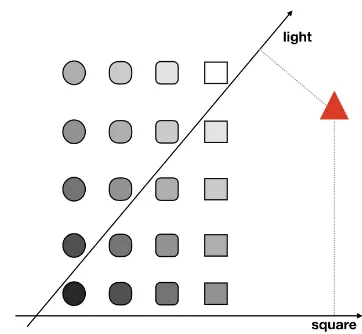
In the aforementioned applications, feature di-rections are typically emerging from vector space representations that have been learned with a similarity-centred objective, i.e. the main consid-eration when learning these representations is that similar objects should be represented as similar vectors. An important observation is that such spaces may not actually be optimal for modelling feature directions. To illustrate why this can be the case, Figure1 shows a toy example in which basic geometric shapes are embedded in a two-dimensional space. Within this space, we can identify directions which encode how light an ob-ject is and how closely its shape resembles a square. While most of the shapes embedded in this space are grey-scale circles and squares, one of the shapes embedded in this space is a red triangle, which is a clear outlier. If this space is learned with a similarity-centred objective, the representation of the triangle will be far from all the other shapes. However, this means that out-liers like this will often take up extreme positions in the rankings induced by the feature directions, and may thus lead us to incorrectly assume that they have certain features. In this example, the triangle would incorrectly be considered as the shape which most exhibits the features “light” and “square”. In contrast, if we had learned the repre-sentation with the knowledge that it should model these two features rather than similarity, this trian-gle would have ended up closer to the bottom-left corner.

Unfortunately, we usually have no a priori

knowledge of which are the most salient features. In this paper, we therefore suggest the follow-ing fully unsupervised strategy. First, we learn

Figure 1: Toy example showing the effect of out-liers in a two-dimensional embedding of geomet-ric shapes.

a semantic space from bag-of-words representa-tions of the considered objects, using a standard similarity-centric method. Using the method from (Derrac and Schockaert, 2015), we subsequently determine the most salient features in the consid-ered domain, and their corresponding directions. Finally, we fine-tune the semantic space and the associated feature directions, modelling the con-sidered features in a more faithful way. This last step is the main contribution of this paper. All code and hyperparameters are available online1.

2 Related Work

Topic models. The main idea underlying our method is to learn a representation in terms of salient features, where each of these features is de-scribed using a cluster of natural language terms. This is somewhat similar to Latent Dirichlet Al-location (LDA), which learns a representation of text documents as multinomial distributions over latent topics, where each of these topics corre-sponds to a multinomial distribution over words (Blei et al., 2003). Topics tend to correspond to salient features, and are typically labelled with the most probable words according to the corre-sponding distribution. However, while LDA only uses bag-of-words (BoW) representations, our fo-cus is specifically on identifying and improving features that are modelled as directions in seman-tic spaces. One advantage of using vector spaces is that they offer more flexibility in how

addi-1_{https://github.com/ThomasAger/}

tional information can be taken into account, e.g. they allow us to use neural representation learn-ing methods to obtain these spaces. Many ex-tensions of LDA have been proposed to incorpo-rate additional information as well, e.g. aiming to avoid the need to manually specify the num-ber of topics (Teh et al.,2004), modelling corre-lations between topics (Blei and Lafferty, 2005), or by incorporating meta-data such as authors or time stamps (Rosen-Zvi et al., 2004; Wang and McCallum, 2006). Nonetheless, such techniques for extending LDA offer less flexibility than neu-ral network models, e.g. for exploiting numerical attributes or visual features.

Fine-tuning embeddings. Several authors have looked at approaches for adapting word embed-dings. One possible strategy is to change how the embedding is learned in the first place. For exam-ple, some approaches have been proposed to learn word embeddings that are better suited at captur-ing sentiment Tang et al.(2016), or to learn em-beddings that are optimized for relation extraction Hashimoto et al.(2015). Other approaches, how-ever, start with a pre-trained embedding, which is then modified in a particular way. For example, in (Faruqui et al.,2015) a method is proposed to bring the vectors of semantically related words, as specified in a given lexicon, closer together. Simi-larlyYu et al.(2017) propose a method for refining word vectors to improve how well they model sen-timent. In (Labutov and Lipson,2013) a method is discussed to adapt word embeddings based on a given supervised classification task.

Semantic spaces. Within the field of cogni-tive science, feature representations and semantic spaces both have a long tradition as alternative, and often competing representations of semantic relatedness (Tversky, 1977). Conceptual spaces (G¨ardenfors,2004) to some extent unify these two opposing views, by representing objects as points in vector spaces, one for each facet (e.g. color, shape, taste in a conceptual space of fruit), such that the dimensions of each of these vector spaces correspond to primitive features. The main appeal of conceptual spaces stems from the fact that they allow a wide range of cognitive and linguistic phe-nomena to be modelled in an elegant way. The idea of learning semantic spaces with accurate fea-ture directions can be seen as a first step towards methods for learning conceptual space representa-tions from data, and thus towards the use of more

cognitively plausible representations of meaning in computer science. Our method also somewhat relates to the debates in cognitive science on the relationship between similarity and rule based pro-cesses (Hahn and Chater,1998), in the sense that it allows us to explicitly link similarity based cate-gorization methods (e.g. an SVM classifier trained on semantic space representations) with rule based categorization methods (e.g. the decision trees that we will learn from the feature directions).

3 Identifying Feature Directions

We assume that a domain-specific semantic space is given, and that for each of the objects which are modelled in this space, we also have a BoW repre-sentation. Our overall aim is to find directions in the semantic space that model salient features of the considered domain. For example, given a se-mantic space of movies, we would like to find a di-rection that models the extent to which each movie is scary, among others. Such a direction would then allow us to rank movies from the least scary to the most scary. We will refer to such directions asfeature directions. Formally, each feature direc-tion will be modelled as a vectorvf. However, we

refer todirectionsrather thanvectorsto emphasize their intended ordinal meaning: feature directions are aimed at ranking objects rather than e.g. mea-suring degrees of similarity. In particular, if ois the vector representation of a given object then we can think of the dot productvf ·oas the value of

object ofor feature f, and in particular, we take

vf ·o1 < vf ·o2to mean thato2 has the featuref

to a greater extent thano1.

To identify feature directions, we use a variant of the unsupervised method proposed in (Derrac and Schockaert, 2015), which we explain in this section. In Section4, we will then introduce our approach for fine-tuning the semantic space and associated feature directions.

20 Newsgroups: Accuracy Scored Movie Reviews: NDCG Scored Place-types: Kappa Scored

{sins, sinful, jesus, moses} {environmentalist, wildlife, ecological} {smile, kid, young, female} {hitters, catcher, pitching, batting} {prophets, bibles, scriptures} {rust, rusty, broken, mill} {ink, printers, printer, matrix} {assassinating, assasins, assasin} {eerie, spooky, haunted, ghosts} {jupiter, telescope, spacecraft, satellites} {reanimated, undead, zombified} {religious, christian, chapel, carved} {firearm, concealed, handgun, handguns} {ufos, ufo, extraterrestrial, extraterrestrials} {fur, tongue, teeth, ears}

{escaped, terror, wounded, fled} {swordsman, feudal, swordfight, swordplay} {weeds, shed, dirt, gravel} {cellular, phones, phone} {scuba, divers, undersea} {stonework, archway, brickwork} {brake, steering, tires, brakes} {regiment, armys, soliders, infantry} {rails, rail, tracks, railroad} {riders, rider, ride, riding} {toons, animations, animating, animators} {dirty, trash, grunge, graffiti} {formats, jpeg, gif, tiff} {fundamentalists, doctrine, extremists} {tranquility, majestic, picturesque} {physicians, treatments physician} {semitic, semitism, judaism, auschwitz} {monument, site, arch, cemetery} {bacteria, toxic, biology, tissue} {shipwrecked, ashore, shipwreck} {journey, traveling, travelling} {planets, solar, mars, planetary} {planetary, earths, asteroid, spaceships} {mother, mom, children, child} {symptoms, syndrome, diagnosis} {atheism, theological, atheists, agnostic} {frost, snowy, icy, freezing} {universities, nonprofit, institution} {astronaut, nasa, spaceship, astronauts} {colourful, vivid, artistic, vibrant}

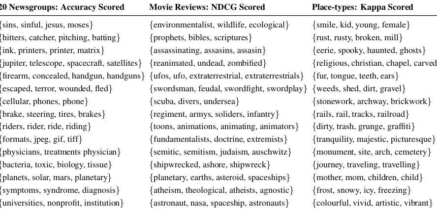
Table 1: The first clustered words of features for three different domains and three different scoring types.

is trained to find a hyperplaneHw in the

seman-tic space that separates objects which containwin their BoW representation from those that do not. The vectorvwperpendicular to this hyperplane is

then taken as the direction that models the wordw.

Step 2: Filtering candidate feature directions. To determine whether the wordwis likely to de-scribe an important feature for the considered do-main, we then evaluate the quality of the candi-date feature directionvw. For example, we can use

the classification accuracy to evaluate the quality in terms of the corresponding logistic regression classifier: if this classifier is sufficiently accurate, it must mean that whether wordwrelates to object

o (i.e. whether it is used in the description of o) is important enough to affect the semantic space representation ofo. In such a case, it seems rea-sonable to assume thatw describes an important feature for the given domain.

One problem with accuracy as a scoring func-tion is that these classificafunc-tion problems are of-ten very imbalanced. In particular, for very rare words, a high accuracy might not necessarily im-ply that the corresponding direction is accurate. For this reason,Derrac and Schockaert(2015) pro-posed to use Cohen’s Kappa score instead. In our experiments, however, we found that accuracy sometimes yields better results, so rather than fix the scoring function, we keep this as a hyperpa-rameter of the model that can be tuned.

In addition to accuracy and Kappa, we also

consider Normalized Discounted Cumulative Gain (NDCG). This is a standard metric in information retrieval which evaluates the quality of a rank-ing w.r.t. some given relevance scores (J¨arvelin and Kek¨al¨ainen, 2002). In our case, the rank-ings of the objects o are those induced by the dot products vw ·o and the relevance scores are

determined by the Pointwise Positive Mutual In-formation (PPMI) scoreppmi(w, o), of the word

w in the BoW representation of object o where

ppmi(w, o) = max 0,log pwo

pw∗·p∗o

, and

pwo=

n(w, o)

P

w0

P

o0n(w0, o0)

where n(w, o) is the number of occurrences of

w in the BoW representation of object o, pw∗ = P

o0p_wo0 and p_∗o = P

w0p_w0_o. In principle,

we may expect that accuracy and Kappa are best suited for binary features, as they rely on a hard separation in the space between objects that have the word in their BoW representation and those that do not, while NDCG should be better suited for gradual features. In practice, however, we could not find such a clear pattern in the differ-ences between the words chosen by these metrics despite often finding different words.

Step 3: clustering candidate feature directions. As the final step, we cluster the best-scoring can-didate feature directions vw. Each of these

clustering step is three-fold: it will ensure that the feature directions are sufficiently different (e.g. in a space of movies there is little point in having

funny and hilarious as separate features), it will make the features easier to interpret (as a clus-ter of clus-terms is more descriptive than an individ-ual term), and it will alleviate sparsity issues when we want to relate features with the BoW represen-tation, which will play an important role for the fine-tuning method described in the next section.

As input to the clustering algorithm, we con-sider theN best-scoring candidate feature direc-tionsvw, whereN is a hyperparameter. To cluster

theseN vectors, we have followed the approach proposed in (Derrac and Schockaert,2015), which we found to perform slightly better thanK-means. The main idea underlying their approach is to se-lect the cluster centers such that (i) they are among the top-scoring candidate feature directions, and (ii) are as close to being orthogonal to each other as possible. We refer to (Derrac and Schockaert, 2015) for more details. The output of this step is a set of clustersC1, ..., CK, where we will

iden-tify each clusterCj with a set of words. We will

furthermore write vCj to denote the centroid of

the directions corresponding to the words in the cluster Cj, which can be computed as vCj =

1

|Cj|

P

wl∈Cjvl provided that the vectors vw are

all normalized. These centroids vC1, ..., vCk are

the feature directions that are identified by our method.

Table1displays some examples of clusters that have been obtained for three of the datasets that will be used in the experiments, modelling respec-tively movies, place-types and newsgroup post-ings. For each dataset, we used the scoring func-tion that led to the best performance on develop-ment data(see Section5). Only the first four words whose direction is closest to the centroid vC are

shown.

4 Fine-Tuning Feature Directions

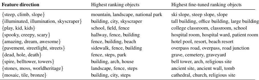
To illustrate that the method from Section 3 can produce sub-optimal directions, the second col-umn of Table2 shows the top-ranked objects for some feature directions in the semantic space of place-types. For the feature represented by the cluster{steep,climb,slope}, the top ranked object

mountain is clearly relevant. However, the next two objects — landscape and national park — are not directly related to this feature. Intuitively,

they are ranked highly because of their similarity tomountainin the vector space. Similarly, for the second feature,buildingis ranked highly because of its similarity to skyscraper, despite intuitively not having this feature. Finally, fencereceived a high rank for several features, mostly because it is an outlier in the space.

To improve the directions and address these problems, we propose a method for fine-tuning the semantic space representations and corresponding feature directions. The main idea is to use the BoW representations of the objects as a kind of weak supervision signal: if an object should be ranked highly for a given feature, we would ex-pect the words describing that feature to appear frequently in its description. In particular, for each feature f we determine a total ordering 4f such

thato4f o0iff the featuref is more prominent in

the BoW represention of objecto0than in the BoW representation ofo. We will refer to4f as the

tar-get rankingfor featuref. If the feature directions are in perfect agreement with this target ranking, it would be the case thato4o0iffvC·o≤vC·o0.

Since this will typically not be the case, we subse-quently determinetarget values for the dot prod-uctsvC ·o. These target values represent the

min-imal way in which the dot products need to be changed to ensure that they respect the target rank-ing. Finally, we use a simple feedforward neural network to adapt the semantic space representa-tionsoand feature directionsvC to make the dot

productsvC·oas close as possible to these target

values.

4.1 Generating Target Rankings

LetC1, ..., CKbe the clusters that were found

us-ing the method from Section 3. Each cluster Ci

typically corresponds to a set of semantically re-lated words {w1, ..., wn}, which describe some

salient feature from the considered domain. From the BoW representations of the objects, we can now define a ranking that reflects how strongly each object is related to the words from this clus-ter. To this end, we represent each object as a bag of clusters (BoC) and then compute PPMI scores over this representation. In particular, for a clusterC ={w1, ..., wm}, we definen(C, o) =

Pm

i=1n(wi, o). In other words,n(C, o)is the

to-tal number of occurrences of words from cluster

C in BoW representation of o. We then write

Feature direction Highest ranking objects Highest fine-tuned ranking objects

{steep, climb, slope} mountain, landscape, national park ski slope, steep slope, slope

{illuminated, illumination, skyscraper} building, city, skyscraper tall building, office building, large building {play, kid, kids} school, field, fence college classroom, classroom, school {spooky, creepy, scary} hallway, fence, building hospital room, hospital ward, patient room {amazing, dream, awesome} fence, building, beach hotel pool, resort, beach resort

{pavement, streetlight, streets} sidewalk, fence, building overpass road, overpass, road junction {dead, hole, death} fence, steps, park grave, cemetery, graveyard

{spire, belltower, towers} building, arch, house bell tower, arch, religious site {stones, moss, worldheritage} landscape, fence, steps ancient site, ancient wall, tomb {mosaic, tile, bronze} building, city, steps cathedral, church, religious site

Table 2: Comparing the highest ranking place-type objects in the original and fine-tuned space.

this BoC representation, which is evaluated in the same way as ppmi(C, o), but using the counts

n(C, o)rather thann(w, o). The target ranking for clusterCiis then such thato1is ranked higher than

o2 iff ppmi(Ci, o1) > ppmi(Ci, o2). By

comput-ing PPMI scores w.r.t. clusters of words, we allevi-ate problems with sparsity and synonymy, which in turn allows us to better estimate the intensity with which a given feature applies to the object. For instance, an object describing a violent movie might not actually mention the word ‘violent’, but would likely mention at least some of the words from the same cluster (e.g. ‘bloody’ ‘brutal’ ‘vi-olence’ ‘gory’). Similarly, this approach allows us to avoid problems with ambiguous word usage; e.g. if a movie is said to contain ‘violent language’, it will not be identified as violent if other words re-lated to this feature are rarely mentioned.

4.2 Generating Target Feature Values

Finding directions in a vector space that induce a set of given target rankings is computationally hard2. Therefore, rather than directly using the target rankings from Section 4.1 to fine-tune the semantic space, we will generate target values for the dot products vCj ·oi from these target

rank-ings. One straightforward approach would be to use the PPMI scoresppmi(Cj, oi). However these

target values would be very different from the ini-tial dot products, which among others means that too much of the similarity structure from the initial vector space would be lost. Instead, we will use isotonic regression to find target valuesτ(Cj, oi)

for the dot productvCj·oi, which respect the

rank-ing induced by the PPMI scores, but otherwise re-main as close as possible to the initial dot

prod-2_{It is complete for the complexity class∃}

R, which sits

between NP and PSPACE (Schockaert and Lee,2015).

ucts.

Let us consider a cluster Cj for which we

want to determine the target feature values. Let

oσ1, ..., oσn be an enumeration of the objects such

that ppmi(Cj, oσi) ≤ ppmi(Cj, oσi+1) for i ∈

{1, ..., n −1}. The corresponding target values

τ(Cj, oi)are then obtained by solving the

follow-ing optimization problem:

Minimize: X

i

(τ(Cj, oi)−vCj·oi) 2

Subject to:

τ(Cj, oσ1)≤τ(Cj, oσ2)≤...≤τ(Cj, oσn)

4.3 Fine-Tuning

We now use the target valuesτ(Cj, oi)to fine-tune

the initial representations. To this end, we use a simple neural network architecture with one hid-den layer. As inputs to the network, we use the initial vectorso1, ..., on ∈ Rk. These are fed into a layer of dimensionl:

hi=f(W oi+b)

whereW is anl×kmatrix,b∈_Rl_{is a bias term,}

andf is an activation function. After training the network, the vectorhi will correspond to the new

representation of the ith_{object. The vectorsh}

iare

finally fed into an output layer containing one neu-ron for each cluster:

gi=Dhi

where D is a K ×l matrix. Note that by using a linear activation in the output layer, we can in-terpret the rows of the matrixDas theK feature directions, with the components of the vectorgi =

20 Newsgroups F1 D1 F1 D3 F1 DN

FT MDS 0.50 0.47 0.44

MDS 0.44 0.42 0.43

FT PCA 0.40 0.36 0.34

PCA 0.25 0.27 0.36

FT Doc2Vec 0.44 0.42 0.41

Doc2Vec 0.29 0.34 0.44

FT AWV 0.47 0.45 0.40

AWV 0.41 0.38 0.43

FT AWVw 0.41 0.41 0.43

AWVw 0.38 0.40 0.43

LDA 0.40 0.37 0.35

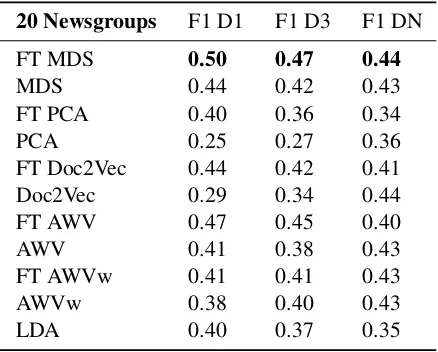
Table 3: Results for 20 Newsgroups.

As the loss function for training the network, we use the squared error between the outputs g_ij and the corresponding target valuesτ(Cj, oi), i.e.:

L=X

i

X

j

(gj_i −τ(Cj, oi))2

The effect of this fine-tuning step is illustrated in the right-most column of Table 2, where we can see that in each case the top ranked objects are now more closely related to the feature, despite being less common, and outliers such as ‘fence’ no longer appear.

5 Evaluation

To evaluate our method, we consider the problem of learning interpretable classifiers. In particu-lar, we learn decision trees which are limited to depth 1 and 3, which use the rankings induced by the feature directions as input. This allows us to simultaneously assess to what extent the method can identify the right features and whether these features are modelled well using the learned di-rections. Note that depth 1 trees are only a sin-gle direction and a cut-off, so to perform well, the method needs to identify a highly relevant feature to the considered category. Depth 3 decision trees are able to model categories that can be character-ized using at most three feature directions.

5.1 Experimental set-up

Datasets. We evaluate our method on four datasets. First, we used themoviesandplace-types

datasets from (Derrac and Schockaert, 2015), which are available in preprocessed form3. The

3_{http://www.cs.cf.ac.uk/}

semanticspaces/

former describes 15000 movies, using a BoW rep-resentation that was obtained by combining re-views from several sources. However, 1022 du-plicate movies were found in the data, which we removed. The associated classification tasks are to predict the movie genres according to IMDB (23 classes), predicting IMDB plot keywords such as ‘suicide’, ‘beach’ or ‘crying’ (100 classes) and predicting age rating certificates such as ‘UK-15’ ‘UK-18’ or ‘USA-R’ (6 classes). All tasks are evaluated as binary classification tasks. We ran-domly split the datasets into 2/3 for training and 1/3 for testing. The place-types dataset was ob-tained by associating each place-type with the bag of tags that have been used to describe places of that type on Flickr. It contains BoW represena-tions for 1383 different place-types. The classi-fication problems for this dataset involve predict-ing whether a place-type belongs to a given cate-gory in three different taxonomies: Geonames (7 classes), Foursquare (9 classes) and OpenCYC (20 classes). Since many of these categories are very small, for this dataset we have used 5-fold cross validation.

The remaining two datasets are standard datasets for document classification: 20 news-groupsand theIMDB sentimentdataset. For the 20 newsgroups dataset, the standard4 split was used where 11314 of the 18446 documents are used for training. Headers, footers and quote metadata were removed using scikit-learn5. The associated classification problem is to predict which news-group a given post was submitted to (20 classes). The IMDB sentiment dataset contains a total of 50000 documents, and it is split into 25000 docu-ments for training and 25000 for testing. For the newsgroups and sentiment datasets, we used stop-words from the NLTK python package (Loper and Bird,2002). For these datasets, we used all (low-ercased) tokens and retained numbers, rather than only using nouns and adjectives. The associated classification problem is to predict the sentiment of the review (positive or negative).

Semantic Spaces. We will consider semantic spaces that have been learned using a number of different methods. First, following (Derrac and Schockaert,2015), we use Multi-Dimensional Scaling (MDS) to learn semantic spaces from the angular differences between the PPMI weighted

4

http://qwone.com/˜jason/20Newsgroups/ 5_{http://scikit-learn.org/stable/}

Movie Reviews

Genres D1 D3 DN Keywords D1 D3 DN Ratings D1 D3 DN

FT MDS 0.57 0.56 0.51 FT MDS 0.33 0.33 0.24 FT MDS 0.49 0.51 0.46

MDS 0.40 0.49 0.52 MDS 0.31 0.32 0.25 MDS 0.46 0.49 0.46

FT AWV 0.42 0.42 0.39 FT AWV 0.25 0.25 0.15 FT AWV 0.47 0.44 0.39

AWV 0.35 0.44 0.43 AWV 0.26 0.21 0.19 AWV 0.44 0.48 0.41

LDA 0.52 0.51 0.45 LDA 0.22 0.19 0.18 LDA 0.48 0.48 0.41

Place-types

Geonames D1 D3 DN Foursquare D1 D3 DN OpenCYC D1 D3 DN

FT MDS 0.32 0.31 0.24 FT MDS 0.41 0.44 0.41 FT MDS 0.35 0.36 0.30

MDS 0.32 0.31 0.21 MDS 0.38 0.42 0.42 MDS 0.35 0.36 0.29

FT AWV 0.31 0.29 0.23 FT AWV 0.39 0.42 0.41 FT AWV 0.37 0.37 0.28

AWV 0.28 0.28 0.22 AWV 0.32 0.37 0.31 AWV 0.33 0.35 0.26

LDA 0.34 0.32 0.27 LDA 0.55 0.48 0.47 LDA 0.40 0.36 0.31

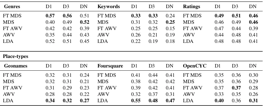
Table 4: The results for Movie Reviews and Place-Types on depth-1, depth-3 and unbounded trees.

IMDB Sentiment D1 D3 DN

FT PCA 0.78 0.80 0.79

PCA 0.76 0.82 0.80

FT AWV 0.72 0.76 0.71

AWV 0.74 0.76 0.71

LDA 0.79 0.80 0.79

Table 5: Results for IMDB Sentiment.

BoW vectors. We also consider PCA, which di-rectly uses the PPMI weighted BoW vectors as input, and which avoids the quadratic complex-ity of the MDS method. As our third method, we consider Doc2vec, which is inspired by the Skip-gram model (Le and Mikolov,2014). Finally, we also learn semantic spaces by averaging word vec-tors, using a pre-trained GloVe word embeddings trained on the Wikipedia 2014 + Gigaword 5 cor-pus6. While simply averaging word vectors may seem naive, this was found to be a competitive ap-proach for unsupervised representations in several applications (Hill et al., 2016). We consider two variants, In the first variant (denoted by AWV), we simply average the vector representations of the words that appear at least twice in the BoW representation, or at least 15 times in the case of the movies dataset. The second variant (denoted by AWVw) uses the same words, but weights the vectors by PPMI score. As a comparison method, we also include results for LDA.

Methodology. As candidate words for learning

6_{https://nlp.stanford.edu/projects/}

glove/

the initial directions, we only consider sufficiently frequent words. The thresholds we used are 100 for the movies dataset, 50 for the place-types, 30 for 20 newsgroups, and 50 for the IMDB senti-ment dataset. We used the logistic regression im-plementation from scikit-learn to find the direc-tions. We deal with class imbalance by weighting the positive instances higher.

For hyperparameter tuning, we take 20% of the data from the training split as development data. We choose the hyperparameter values that maximize the F1 score on this development data. As candidate values for the number of dimen-sions of the vector spaces we used{50,100,200}. The number of directions to be used as in-put to the clustering algorithm was chosen from

To learn the decision trees, we use the scikit-learn implementation of CART, which allows us to limit the depth of the trees. To mitigate the effects of class imbalance, the less frequent class was given a higher weight during training.

5.2 Results

Table 3 shows the results for the 20 newsgroups dataset, where we use FT to indicate the results with fine-tuning7. We can see that the fine-tuning method consistently improves the performance of the depth-1 and depth-3 trees, often in a very sub-stantial way. After fine-tuning, the results are also consistently better than those of LDA. For the unbounded trees (DN), the differences are small and fine-tuning sometimes even makes the re-sults worse. This can be explained by the fact that the fine-tuning method specializes the space towards the selected features, which means that some of the structure of the initial space will be distorted. Unbounded decision trees are far less sensitive to the quality of the directions, and can even perform reasonably on random direc-tions. Interestingly, depth-1 trees achieved the best overall performance, with depth-3 trees and es-pecially unbounded trees overfitting. Since MDS and AWV perform best, we have only considered these two representations (along with LDA) for the remaining datasets, except for the IMDB Sen-timent dataset, which is too large for using MDS.

The results for the movies and place-types datasets are shown in Table4. For the MDS rep-resentations, the fine-tuning method again con-sistently improved the results for D1 and D3 trees. For the AWV representations, the fine-tuning method was also effective in most cases, al-though there are a few exceptions. What is notice-able is that for movie genres, the improvement is substantial, which reflects the fact that genres are a salient property of movies. For example, the deci-sion tree for the genre ‘Horror’ could use the fea-ture direction for{gore,gory,horror,gruesome}. Some of the other datasets refer to more spe-cialized properties, and the performance of our method then depends on whether it has identified features that relate to these properties. It can be expected that a supervised variant of this method would perform consistently better in such cases.

7_{Since the main purpose of this first experiment was to}

see whether fine-tuning improved consistently across a broad set of representations, here we considered a slightly reduced pool of parameter values for hyperparameter tuning.

After fine-tuning, the MDS based representation outperforms LDA on the movies dataset, but not for the place-types. This is a consequence of the fact that some of the place-type categories refer to very particular properties, such as geological phe-nomena, which may not be particularly dominant among the Flickr tags that were used to generate the spaces. In such cases, using a BoW based rep-resentation may be more suitable.

Finally, the results for IMDB Sentiment are shown in Table 5. In this case, the fine-tuning method fails to make meaningful improvements, and in some cases actually leads to worse re-sults. This can be explained from the fact that the feature directions which were found for this space are themes and properties, rather than as-pects of binary sentiment evaluation. The fine-tuning method aims to improve the representa-tion of these properties, possibly at the expense of other aspects.

6 Conclusions

We have introduced a method to identify and model the salient features from a given domain as directions in a semantic space. Our method is based on the observation that there is a trade-off between accurately modelling similarity in a vector space, and faithfully modelling features as directions. In particular, we introduced a post-processing step, modifying the initial semantic space, which allows us to find higher-quality di-rections. We provided qualitative examples that illustrate the effect of this fine-tuning step, and quantitatively evaluated its performance in a num-ber of different domains, and for different types of semantic space representations. We found that after fine-tuning, the feature directions model the objects in a more meaningful way. This was shown in terms of an improved performance of low-depth decision trees in natural categorization tasks. However, we also found that when the con-sidered categories are too specialized, the fine-tuning method was less effective, and in some cases even led to a slight deterioration of the re-sults. We speculate that performance could be im-proved for such categories by integrating domain knowledge into the fine-tuning method.

Acknowledgments

References

David M. Blei and John D. Lafferty. 2005. Correlated topic models. In Advances in Neural Information Processing Systems 18, pages 147–154.

David M. Blei, Andrew Y. Ng, Michael I. Jordan, and John Lafferty. 2003. Latent dirichlet allocation.

Journal of Machine Learning Research, 3:2003.

Antoine Bordes, Nicolas Usunier, Jason Weston, and Oksana Yakhnenko. 2013. Translating embeddings for modeling multi-relational data. InIn Advances in Neural Information Processing Systems 26. Cur-ran Associates, Inc, pages 2787–2795.

Berkan Demirel, Ramazan Gokberk Cinbis, and Nazli Ikizler-Cinbis. 2017. Attributes2classname: A dis-criminative model for attribute-based unsupervised zero-shot learning. In IEEE International Confer-ence on Computer Vision, pages 1241–1250.

J. Derrac and S. Schockaert. 2015. Inducing seman-tic relations from conceptual spaces: a data-driven approach to plausible reasoning. Artificial Intelli-gence, pages 74–105.

John Duchi, Elad Hazan, and Yoram Singer. 2011. Adaptive Subgradient Methods for Online Learning and Stochastic Optimization. Journal of Machine Learning Research, 12:2121–2159.

Manaal Faruqui, Jesse Dodge, Sujay Kumar Jauhar, Chris Dyer, Eduard Hovy, and Noah A Smith. 2015. Retrofitting word vectors to semantic lexicons. In

Proceedings of the 2015 Conference of the North American Chapter of the Association for Computa-tional Linguistics: Human Language Technologies, pages 1606–1615.

Peter G¨ardenfors. 2004. Conceptual Spaces: The Ge-ometry of Thought. MIT press.

Abhijeet Gupta, Gemma Boleda, Marco Baroni, and Sebastian Pad. 2015. Distributional vectors encode referential attributes. In Proceedings of the 2015 Conference on Empirical Methods in Natural Lan-guage Processing.

Ulrike Hahn and Nick Chater. 1998. Similarity and rules: distinct? exhaustive? empirically distinguish-able? Cognition, 65:197 – 230.

Kazuma Hashimoto, Pontus Stenetorp, Makoto Miwa, and Yoshimasa Tsuruoka. 2015. Task-oriented learning of word embeddings for semantic relation classification. CoRR, abs/1503.00095.

Felix Hill, Kyunghyun Cho, and Anna Korhonen. 2016. Learning distributed representations of sentences from unlabelled data. In Proceedings of the 2016 Conference of the North American Chapter of the Association for Computational Linguistics: Human Language Technologies, pages 1367–1377.

Shoaib Jameel, Zied Bouraoui, and Steven Schockaert. 2017. Member: Max-margin based embeddings for entity retrieval. InProceedings of the 40th Interna-tional ACM SIGIR Conference on Research and De-velopment in Information Retrieval, pages 783–792.

Kalervo J¨arvelin and Jaana Kek¨al¨ainen. 2002. Cumu-lated gain-based evaluation of IR techniques. ACM Transactions on Information Systems, 20(4):422– 446.

Joo-Kyung Kim and Marie-Catherine de Marneffe. 2013. Deriving adjectival scales from continuous space word representations. In Proceedings of the 2013 Conference on Empirical Methods in Natural Language Processing, pages 1625–1630. ACL.

Adriana Kovashka, Devi Parikh, and Kristen Grauman. 2012. Whittlesearch: Image search with relative at-tribute feedback. InIEEE Conference on Computer Vision and Pattern Recognition, pages 2973–2980.

Igor Labutov and Hod Lipson. 2013. Re-embedding words. In Proceedings of the 51st Annual Meet-ing of the Association for Computational LMeet-inguis- Linguis-tics, pages 489–493.

Quoc V. Le and Tomas Mikolov. 2014. Distributed rep-resentations of sentences and documents. In Pro-ceedings of the 31th International Conference on Machine Learning, pages 1188–1196.

Dawen Liang, Jaan Altosaar, Laurent Charlin, and David M Blei. 2016. Factorization meets the item embedding: Regularizing matrix factorization with item co-occurrence. In Proceedings of the 10th ACM Conference on Recommender Systems, pages 59–66.

Edward Loper and Steven Bird. 2002. NLTK: The nat-ural language toolkit. InProceedings of the ACL-02 Workshop on Effective Tools and Methodologies for Teaching Natural Language Processing and Compu-tational Linguistics, pages 63–70.

Tomas Mikolov, Ilya Sutskever, Kai Chen, Greg Cor-rado, and Jeffrey Dean. 2013. Distributed represen-tations of words and phrases and their composition-ality. InProceedings of the 26th International Conference on Neural Information Processing Systems -Volume 2, NIPS’13, pages 3111–3119, USA. Curran Associates Inc.

Jeffrey Pennington, Richard Socher, and Christopher Manning. 2014. Glove: Global vectors for word representation. In Proceedings of the 2014 Con-ference on Empirical Methods in Natural Language Processing (EMNLP), pages 1532–1543. Associa-tion for ComputaAssocia-tional Linguistics.

Sascha Rothe and Hinrich Sch¨utze. 2016. Word embedding calculus in meaningful ultradense sub-spaces. InACL (2). The Association for Computer Linguistics.

Steven Schockaert and Jae Hee Lee. 2015. Qualita-tive reasoning about directions in semantic spaces. In Proceedings of the Twenty-Fourth International Joint Conference on Artificial Intelligence, pages 3207–3213. AAAI Press.

Duyu Tang, Furu Wei, Bing Qin, Nan Yang, Ting Liu, and Ming Zhou. 2016. Sentiment embeddings with applications to sentiment analysis. IEEE Transac-tions on Knowledge and Data Engineering, 28:496– 509.

Yee Whye Teh, Michael I. Jordan, Matthew J. Beal, and David M. Blei. 2004. Sharing clusters among related groups: Hierarchical dirichlet processes. In

Proceedings of the 17th International Conference on Neural Information Processing Systems, NIPS’04, pages 1385–1392, Cambridge, MA, USA. MIT Press.

Amos Tversky. 1977. Features of similarity. Psycho-logical review, 84:327–352.

Christophe Van Gysel, Maarten de Rijke, and Evange-los Kanoulas. 2016. Learning latent vector spaces for product search. In Proceedings of the 25th ACM International on Conference on Information and Knowledge Management, pages 165–174.

Christophe Van Gysel, Maarten de Rijke, and Evange-los Kanoulas. 2017. Structural regularities in text-based entity vector spaces. In Proceedings of the ACM SIGIR International Conference on Theory of Information Retrieval, pages 3–10.

Flavian Vasile, Elena Smirnova, and Alexis Conneau. 2016. Meta-prod2vec: Product embeddings using side-information for recommendation. In Proceed-ings of the 10th ACM Conference on Recommender Systems, pages 225–232.

Paolo Viappiani, Boi Faltings, and Pearl Pu. 2006. Preference-based search using example-critiquing with suggestions. Journal of Artificial Intelligence Research, 27:465–503.

Jesse Vig, Shilad Sen, and John Riedl. 2012. The tag genome: Encoding community knowledge to sup-port novel interaction. ACM Transactions on Inter-active Intelligent Systems, 2(3):13:1–13:44.

Xuerui Wang and Andrew McCallum. 2006. Topics over time: a non-markov continuous-time model of topical trends. In Proceedings of the 12th ACM SIGKDD international conference on Knowledge discovery and data mining, pages 424–433. ACM.