Abstract—Skewing of the scanned image is an inevitable process and its detection is an important issue for document recognition systems. The skew of the scanned document image specifies the deviation of the text lines from the horizontal or vertical axis. This paper surveys methods to detect this skew in two steps, dimension reduction and skew estimation. These methods include projection profile analysis, Hough Transform, nearest neighbor clustering, cross-correlation, piece-wise painting algorithm, piece-wise covering by parallelogram, transition counts, morphology.
Index Terms—Document recognition systems, preprocessing, skew, dimension reduction, skew estimation
I. INTRODUCTION
kew detection of scanned document images is one of the most important stages of its recognition preprocessing. The skew of the scanned document image specifies the deviation of its text lines from the horizontal or vertical axis. The skew of the document image can be a global (all document’s blocks have the same orientation), multiple (document’s blocks have a different orientation) or non-uniform (multiple orientation in a text line) [1]. Generally, dimension reduction and skew estimation are two steps of the skew detection of scanned document images. We describe these two steps later.
The first step of skew detection is dimension reduction. Each image is a point in the image space. Each dimension of the image space is related to one of its pixels. The first set of features that can be considered for an image is its pixel values. In other words, the value of each image pixel is one of its features. The dimension of images is high and the employment of all image pixels as its features creates complexity and high computational cost on the irrelevant features. Dimension reduction is the process of reducing the size of features or image pixels and finding another feature with much lower dimensions. We extract or select relevant features of an image with low dimensions from image pixels. To solve a particular problem, we choose several features to achieve the final goal. Features of scanned documents can be divided into three groups:
1. Irrelevant features: those features which are not necessary at all to achieve the desired goal.
Manuscript received Jan 10, 2013; revised Jan 29, 2013.
Sepideh Barekat Rezaei is an M.Sc. student with the Department of Computer Engineering, Faculty of Engineering, Kharazmi University, Tehran, I.R. Iran (e-mail: [email protected]).
Abdolhossein Sarrafzadeh is an Associate Professor and Head of Department of Computing, Unitec Institute of Technology, New Zealand (email: [email protected]).
Jamshid Shanbehzadeh is an Associate Professor with the Department of Computer Engineering, Faculty of Engineering, Kharazmi University (Tarbiat Moallem University of Tehran), Tehran, I.R. Iran (phone: +98 26 34550002; fax: +98 26 34569555; e-mail: [email protected]).
2. Weakly relevant features: features that are not always necessary to achieve the desired goal, but may become necessary in certain conditions. These features can be divided into two categories: redundant and non-redundant features.
3. Strongly relevant features: those features which are always necessary to achieve the desired goal. Dimension reduction methods can be divided into:
1. Feature transformation: in this method, initial set of features transforms to the other set, in respect to retaining the information as much as possible. These methods can be placed in two categories:
a. Feature extraction: in this method, a new set of features is created by the initial feature set . b. Feature generation: in this method, the missing
information detected and added to the feature set. 2. Feature selection: this method select an optimal
subset of features based on an objective function. The optimal subset includes all of the strongly relevant and weakly relevant but non-redundant features.
Different dimension reduction methods can be used in skew detection of scanned document images. One or more methods can be used consecutively. At the end of this phase, a criterion function for skew detection is obtained.
The second step of skew detection is skew estimation. In this step, using the function defined in the previous step, the skew is estimated. The angle corresponding to the maximum or the minimum value of the function is usually considered as the skew. So, in this step, the maximum or the minimum of the criterion function is achieved.
Until now, many methods for skew detection of scanned document images have been proposed. These methods include projection profile analysis, Hough transform, nearest neighbor clustering, cross-correlation, piece-wise painting algorithm, piece-wise covering by parallelogram, transition counts, morphology. In the following section, we describe these methods and explain the features are used, reason for that feature’s suitability for skew detection, the steps of the methods and the history of innovation and change.
II. SKEW DETECTION OF SCANNED DOCUMENT IMAGES A. Projection Profile Analysis
In this method, the horizontal or vertical projection profile is used as a suitable feature for skew detection. Horizontal (or vertical) projection profile is the histogram of a one-dimensional array with a number of entries equal to the number of rows (or columns). The number of black pixels in a row (or column) is stored in the corresponding entry.
When the skew of the document image is zero degrees, the projection profile peak times will be longer. To understand the reason, consider the scan lines are drawn on
Skew Detection of Scanned Document Images
Sepideh Barekat Rezaei, Abdolhossein Sarrafzadeh, and Jamshid Shanbehzadeh
two document image with 5 and zero degrees of skew. Here, the scan line means a row of the image. Scan lines plotted on document image with 5 degrees of skew, include white areas between text lines, while most of scan lines plotted on document image with zero degrees of skew, include a text line and no white areas between text lines. So, in those rows of the image with zero degrees of skew, the number of black pixels is higher and the projection profile peaks are longer. Therefore, the projection profile can be used as a suitable feature for skew detection. We need to create a feature to describe which one is more peaked for comparing peaks of projection profiles. So employing a criterion function provides a numerical description of the peaks. The projection profile analysis process is as follows:
1. Dimension reduction: rotate the binary input image to different angles and at any angle do "a" and "b". a. Feature extraction: obtain the projection profile. b. Feature extraction: calculate criterion function. 2. Skew estimation: obtain the angle corresponding to
the maximum value of criterion function.
In 1988, Postl used the horizontal projection profile for skew detection. He used the sum of squared differences between adjacent elements of the projection profile as the criterion function [2].
In 1993, Bloomberg and Kopec employed the variance of the number of black pixels in each row as the criterion function values. They added a feature selection sub-step before calculating the projection profile and downsampling the image, to reduce the computational burden of this method [3]. In downsampling of the image, the number of image rows and columns are selected. Therefore, image downsampling is a feature selection sub-step.
In the dimension reduction step, the image is rotated to different angles. These angles are the possible skew and determine the search space. In 1995, Bloomberg and his colleagues, in order to reduce the search space dimension, added a feature selection sub-step to the beginning of the dimension reduction step [4]. The input of this sub-step is the whole search space and the output is a small selected part of the whole search space that the skew put in it. In this sub-step, they calculate the projection profile for a sequence of angles. A range around the angle that maximized the criterion function is the output range of this sub-step. With the implementation of the algorithm based on this range, higher resolution can be achieved.
In 1999, Kavallieratou and his colleagues used the horizontal projection profile and several time-frequency distribution of Cohen’s class to skew detection [5]. They added a feature extraction sub-step between "a" and "b" in the dimension reduction step and calculated Cohen’s distribution of projection profile. They used the histogram of maximum intensity of each distribution as a suitable feature for skew detection, and they obtained the angle corresponding to the maximum value of that histogram as the skew. They show that Wigner-Ville distribution, in terms of accuracy and computational time, is better than other distributions of Cohen’s class.
In 2007, Li and colleagues used the two-dimensional discrete wavelet transform to improve the accuracy of the projection profile analysis method. They added a feature extraction sub-step to the dimension reduction step and,
using wavelet transform, decomposed the input image into four sub-bands. Then, they formed the matrix by the absolute values of horizontal approximation sub-band coefficient [6]. The coefficients matrix of each of the four sub-bands can be considered as an image. The dimension of each of these four images is a fourth dimension of the input image. Also, each of the four images has some of the information of the input image. So, obtaining the wavelet transform is a feature extraction sub-step of the dimension reduction step. Since the image corresponding to the horizontal approximation contains information about how to get the text lines, this image can be used as a suitable feature for skew detection of the input image.
In 2009, Sadri and Cheriet reduced the number of local minimums and maximums of the projection profile. Then, they calculated the sum of local maximum heights and the sum of local minimum heights and considered the difference between them as a criterion function [7]. In order to accelerate the search and reduce the computational load, they used a particle swarm optimization algorithm in the second step of the projection profile analysis to find the maximum of the criterion function. Optimization means choosing the best member of a data set. To detect the skew, the best angle must be chosen between the angles of the search space to maximize the criterion function. Criterion function value of each angle can be considered as an angle fitness. In this case, the best angle is the angle that maximizes the criterion function. Thus, the problem of finding the global maximum of the criterion function is defined to choose the best angle between the angles of the search space. Thus, this problem can be considered a one-dimensional optimization problem. So the particle swarm optimization algorithm can be used to solve this problem.
In 2011, Papandreou and Gatos used vertical projection profile for skew detection. They considered the sum of squares of the projection profile elements as the value of the criterion function. This method is robust to noise and warp of the image. This method also works well for the languages where most of their letters include at least one vertical line, such as languages with Latin alphabets [8].
B. Hough Transform
In this method, the straight lines corresponding to the image text lines are extracted as features for skew detection using Hough Transform. Deviation of image text lines from the horizontal or vertical axis is specified as its skew. Therefore, the image text lines can be used as a suitable feature for skew detection. On the other hand, the text lines have the features of straight lines, so Hough Transform can be used to find text lines, and thus to detect the skew. Hough Transform-based method has the following steps:
1. Dimension reduction: do "a" and "b" for the binary input image.
a. Feature extraction: using the Hough Transform to find the text lines of the image.
b. Feature extraction: calculate the criterion function for the angle θ.
2. Skew estimation: obtain the angle corresponding to the maximum value of criterion function.
between 0 and 180 degrees. He considered the rate of change in the accumulator array values for each angle θ as a criterion function of the angle [9].
In 1990, Hinds, in order to reduce the computational cost, added a feature extraction sub-step to the beginning of the dimension reduction step and used run-length encoding for reducing the amount of data. He produced a horizontal and vertical burst image. By using the burst images, emphasis is placed on the bottom of the text lines, and a more accurate skew detection is provided [10].
In 1996, Yu and Jain introduced the hierarchical Hough Transform approach [11]. In the method proposed by Yu and Jain, in order to reduce the dimension of the search space, they performed a feature selection step. At this step, the range of angle θ is divided into large distance and the angle is obtained using Hough Transform. The interval around that angle is the desired output. After this stage, the Hough Transform is performed on the new search space. This new range is divided into small intervals and the final angle is obtained using Hough Transform.
In 2000, Amin and Fischer added a feature selection sub-step to the dimension reduction sub-step and extracted the image connected components and rectangle covers to reduce the computational burden of the Hough Transform method. They grouped them so that adjacent connected components with the same dimensions were considered in the same group. Thus, the image was divided into blocks and each block included connected components within a group. After that, they estimated the skew of each block. For this purpose, they divided each block into vertical sections with a width approximately equal to the width of a connected component. In each section, they kept only the lowest rectangle. They applied Hough Transform to the center of the rectangles. After calculating the skew of each block, they considered a weight for each angle equal to the number of points used in the calculating then classified them. They identified the group with the highest number of angles and considered the average of the angles as the skew [12].
In 2011, Epshtein presented a Hough Transform based method that instead of estimating the direction of text lines, it estimated the direction of the white space between lines [13]. In 2012, Kumar and Singh applied Hough Transform on a set of pixels. Thus, they reduced the running time and maintained the accuracy of the method. They divided the spectrum of the Hough Transform space (the skew can be between 0 and 45 degrees) to the distance by one tenth. Then, they selected the section including the final skew. Finally, they divided that section to the distance by one tenth and searched that for final skew [14].
C. Nearest Neighbors Clustering
In this method, vectors connecting the image connected components to the nearest neighbors are used as features for skew detection. Nearest neighbors of each connected component are usually adjacent letters on the same text line. Therefore, the vectors connecting any connected component to its nearest neighbors are usually characterized by a line parallel to a text line. Since the deviation of the text lines from the horizontal or vertical axis defines the skew, text lines and parallel lines to them can be used as a convenience feature for skew detection. Therefore, those vectors can be
used as features for skew detection. This method can be summarized as follows:
1. Dimension reduction: do "a", "b" and "c" for the input binary image.
a. Feature selection: obtain the connected components.
b. Feature extraction: determine the nearest neighbor set of each connected component. Obtain angle of vectors connecting each component to its nearest neighbor.
c. Feature extraction: calculate the value of the criterion function.
2. Skew estimation: obtain the angle corresponding to the maximum value of criterion function.
In 1986, Hashizume proposed the nearest neighbor clustering method for skew detection. He used just the vector connecting the connected component to its first nearest neighbor. Hashizume used the vector angle histogram as the criterion function [15].
In 1993, O'Gorman developed Hashizume’s method further. He used the vectors connecting each component to its k nearest neighbor [16]. When only the vector connecting the connected component to its first nearest neighbor is used, since it is possible that the first nearest neighbor was noise or subdivision (e.g. point of the letter "i"), the risk of skew detection would be highly improper. Therefore, the method proposed by O'Gorman is more accurate than the method proposed by Hashizume. But the value of k influences the accuracy of the method. If k is large enough, the connected component corresponding to the letters of two or more text lines indicates each other’s closest neighbors are determined, and the accuracy of this method decreases.
In 1999, Jiang proposed focused nearest-neighbor clustering to detect skew. He added a feature selection sub-step after determining connected components and the nearest neighbors, and selected a subset of nearest neighbors. Then, in a feature extraction stage, performed the least squares line fitting for selected neighbors. Finally, like to original method drew the histogram of obtained lines and considered that maximum as skew of document image [17].
In 2001, Liolios placed connected components that belonged to a text line in a cluster. He performed the least squares fitting line for those connected components. Since the larger clusters correspond to the longer text lines, these clusters lead to a better estimation of the skew. So Liolios weighted the obtained angle for each cluster by the number of components within the cluster. Then, he calculated the weighted average of angles and assessment arc tangent of the obtained value as the skew [18].
D. Cross-correlation
In this method, the cross-correlation function is used for skew detection. Similar to Fig. 1, consider the two vertical lines and in locations and . Cross-correlation between the two lines is defined as follows:
, ∑ , , (1)
Whenever the value of , and ,
grow larger, the result of their multiplication is greater. Whenever the multiplication of , and ,
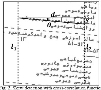
for all values of becomes larger, the value of cross-correlation function between the two lines is greater. Large values of , and , correspond to the light image pixels. Most of the light image pixels are the pixels between the lines. So, if for most values of , , and , correspond to the light pixels between the lines, the cross-correlation function between the two lines is greater. This happens when is equal to the distance between two text lines. It is clear in Fig. 1. Taking the distance between two text lines and between two imaginary vertical lines, the text line angle from the horizontal axis can be found. To understand how to calculate this angle, note the black triangle in Fig. 2. One side of the triangle is the distance between two text lines, and the other side is the distance between the two imaginary vertical lines. Angle θ shown in the triangle is the angle of the text line with the horizontal axis and can be calculated as ⁄ . This angle is the skew of document image. Thus, the cross-correlation function can be used to detect the skew.
In 1993, Yan used cross-correlation function skew detection for the first time [22]. Yan’s method is as follows:
1. Dimension reduction: do "a" and "b" for a range of s. a. Feature extraction: calculate cross-correlation
between the two vertical lines with a certain distance in place of and .
b. Feature extraction: calculate the total cross-correlation functions according to
∑ , (2)
Consider as the value of cost function in s. 2. Skew estimation: find the s that maximize the cost
function. Then estimate the skew as follows:
⁄ (3)
Such a method’s problems include:
1. Calculating the cross-correlation function for the whole image is relatively time-consuming.
2. Vertical image or text decreases its accuracy.
In 1997, Chundhuri, instead of finding the correlation for the entire image, calculated it for small randomly chosen areas. For this purpose, he added a feature selection sub-step to the dimension reduction step and used Monte-Carlo sampling to determine the number of regions to calculate the correlation. He considered the median maximum cross-correlation as the criterion to obtain the skew [23].
In 1999, Chen, like Chundhuri’s method, calculated correlations for a randomly selected small area, but added the verification stage to determine the suitability of the area. Also, in order to solve the second problem of Yan’s method, he calculated horizontal and vertical cross-correlations of the image [24]. For the horizontal text, the vertical cross-correlation function and for the vertical text, the horizontal cross-correlation function had more specific peaks. Whichever cross-correlation function had considerably more specific peaks was more precise at finding its maximum. So, Chen, by selecting the cross-correlation function with more specific peaks, increased the accuracy of Yan’s method.
E. Piece-wise Painting Algorithm (PPA)
In 2011, Alaei introduced the Piece-wise Painting Algorithm (PPA) and used it for segmentation of handwriting texts [25]. He then developed the algorithm for skew detection [26]. If a rectangle is rotated, the angle of a side crossing an axis is equal to the angle that the side perpendicular to that side makes with the axis perpendicular to that axis. So, if the document original rectangle is extracted, we can estimate the skew of the image. PPA can be obtained this rectangle. This process is as follows:
1. Dimension reduction:
a. Feature extraction: run PPA horizontally and vertically. Obtain the bands, length and location of them in the each painted image. Specify candidate bands for each image. Candidate bands form the original rectangle of the document. b. Feature extraction: calculate the slope of 4
regression lines obtained from the starting and middle points of vertical and horizontal candidate bands and 3 straight lines drawn using the starting and middle points of vertical candidate bands and the starting points of horizontal candidate bands. c. Feature extraction: obtain criterion function
values for each of the 7 slope as follows:
, , , , , , (4)
(5) , 1,2, . . ,7 (6)
[image:4.595.62.261.118.280.2]2. Skew estimation: obtain the angle corresponding to the minimum value of .
[image:4.595.82.250.558.708.2]F. Piece-wise Covering by Parallelogram
In 2007, Chou and colleagues proposed this method for skew detection [27]. The document contains a large number of rectangular objects including text lines, text areas, forms, tables, and etc. When the document image skew is zero, all objects can be covered by the rectangles, and when the skew is not zero, objects can be covered by the parallelogram. The skew of the parallelograms is equal to the skew of the document. So, if we create parallelograms at all angles and select a situation in which the objects are best covered, we find the document skew. This method is as follows:
1. Dimension reduction: divide the input binary image into non-overlapping regions, some vertically. These areas are called slabs. Draw the scan lines at all angles. Any part of a scan line in a slab is called a section. For each angle, do "a" and "b".
a. Feature extraction: if a section contains at least one black pixel, gray that. Otherwise, leave it without change. The parallelogram can be drawn. b. Feature extraction: put the area of the gray
parallelogram formed at any angle in . Subtract from the area of document image ( ) and thus calculate the area of parallelograms which complement, , as follows:
(7) 2. Skew estimation: obtain the angle corresponding to
the maximum value of .
In this method, the angle by which the complementary parallelogram regions are larger is used as the skew. An efficient technique for obtaining , is to count the number of white sections in text lines drawn at any angle . To do this, if you have no black pixels in a section, add one unit to the number of white sections.
Chou and colleagues limited searching for the skew to the range of -15 to +15 degrees. To reduce the processing time, instead of searching through all the angles of this period, they performed the following procedure:
1.Search for the best angle in the interval 15°, 15° that is divided by two degrees step size;
2.Choosing the best angle between 1, and 1; 3.Search for the best angle in the interval 1, 1
is divided by 0.1 degrees of step size.
In 2010, Mascaro and his colleagues improved this method in three contexts: getting the size of parallelogram complementary regions, efficient searching for the best angle, preventing undesirable interference caused by components such as noise and vertical separator [28]. In 2012, Na and Jinxiao improved this method, so it could be used for the documents with horizontal orientation [29]. They determined the width of the beam by the image size. Also, they used the threshold T to decide between graying a section and leaving it unchanged.
G. Transition Counts
This method uses the variance of the transition counts as a suitable feature for skew detection. Transition count of a scan line is defined by the number of transitions from black to white or white to black pixels. If transition counts are calculated along parallel lines with text lines, its variance in text regions is bigger than non-text regions. So, using this parameter, text regions can be specified and the skew
estimated.
In 1993, Ishitani for first time used this method to estimate the skew of a document image [30]. Her method is:
1. Dimension reduction: do "a", "b" and "c" for a range of angles relative to the horizontal line.
a. Feature selection: draw scan lines parallel to each other that cover the total document image. b. Feature extraction: count the transitions in each
scan line and put it in .
c. Feature extraction: calculate the mean of transition counts ( ) and their variance for the scan lines with angle , as follows:
1⁄ ∑ (8)
1⁄ ∑ (9)
2. Skew estimation: obtain the angle corresponding to the maximum value of .
In 2000, Chen and Wang used the variance of the transition counts for estimating the skew and determining the page orientation [31]. They added the feature selection sub-step before calculating the variance and selected the region of the image containing enough text. For determining the page orientation, they calculated the variance of the horizontal and vertical transition counts in the range of angles. If the maximum of variance in the horizontal direction is greater than the vertical direction, the page is row-wise and the skew is the angle corresponding to it in the horizontal direction. Otherwise, the page is column-wise and the skew is the angle corresponding to the maximum variance in the vertical direction.
H. Morphology
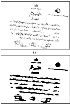
In this method, the image text lines are extracted as suitable features for skew detection using morphological operators. In this method, fill the space between the characters by using morphological operators. Thus, any text lines are black blocks. One of the morphological operators which can be used for this purpose is closing. For example, a document image with 5 degrees skew and a result of performing closing with a 70×30 structural element are shown in Fig. 3.
Fig. 3. (a) A document image with 5 degree skew, (b) result of performing closing on the (a) with 70×30 structural element.
(a)
[image:5.595.357.503.536.753.2]Different methods based on morphology are proposed for skew detection [32]-[35]. For the first time, in 1994, Chen and Haralick used recursive morphological transforms to detect skew [32]. Their proposed procedure is as follows:
1. Dimension reduction:
a. Feature selection: sampling from the input image. b. Feature extraction: fill the space between
characters using recursive closing transforms. Delete ascenders and descenders using recursive opening transforms. Run connected component labeling and then the least squares line fitting. c. Feature selection: calculate the median ( )
and median of variances ( ) of the line’s direction. Take an interval around with the size proportion of . Then make up a subset of the lines in its direction in the interval. This is repeated until and converge.
2. Skew estimation: calculate Bayesian estimation of the skew.
REFERENCES
[1] O. Okun, M. Pietikäinen, and J. Sauvola, “Document skew estimation without angle range restriction,” International Journal on Document Analysis and Recognition, vol. 2, pp. 132-144, 1999.
[2] W. Postl, “Method for automatic correction of character skew in the acquisition of a text original in the form of digital scan results,” United States Patent, 1988.
[3] D. S. Bloomberg and G. E. Kopec, “Method and apparatus for identification and correction of document skew,” United States Patent, 1993.
[4] D. S. Bloomberg, G. E. Kopec, L. Dasari, and H. S. Baird, “Measuring document image skew and orientation,” presented at the Society of Photo-Optical Instrumentation Engineers (SPIE) Conference Series, 1995.
[5] E. Kavallieratou, N. Fakotakis, and G. Kokkinakis, “Skew angle estimation in document processing using Cohen’s class distributions,” Pattern Recognition Letters, vol. 20, pp. 1305-1311, 1999.
[6] S. Li, Q. Shen, and J. Sun, “Skew detection using wavelet decomposition and projection profile analysis,” Pattern Recognition Letters, vol. 28, pp. 555-562, 2007.
[7] J. Sadri and M. Cheriet, “A New Approach for Skew Correction of Documents Based on Particle Swarm Optimization,” in Document Analysis and Recognition, 2009. ICDAR '09. 10th International Conference on Document Analysis and Recognition, 2009, pp. 1066-1070.
[8] A. Papandreou and B. Gatos, “A Novel Skew Detection Technique Based on Vertical Projections,” in Document Analysis and Recognition (ICDAR), 2011 International Conference on Document Analysis and Recognition, 2011, pp. 384-388.
[9] S. N. Srihari and V. Govindaraju, “Analysis of textual images using the Hough transform,” Machine Vision and Applications, vol. 2, pp. 141-153, 1989.
[10] S. C. Hinds, J. L. Fisher, and D. P. D'Amato, “A document skew detection method using run-length encoding and the Hough transform,” in Pattern Recognition, 1990. Proceedings., 10th International Conference on Pattern Recognition, 1990, pp. 464-468 vol.1.
[11] B. Yu and A. K. Jain, “A robust and fast skew detection algorithm for generic documents,” Pattern Recognition, vol. 29, pp. 1599-1629, 1996.
[12] A. Amin and S. Fischer, “A Document Skew Detection Method Using the Hough Transform,” Pattern Analysis & Applications, vol. 3, pp. 243-253, 2000.
[13] B. Epshtein, “Determining Document Skew Using Inter-line Spaces,” in Document Analysis and Recognition (ICDAR), 2011 International Conference, 2011, pp. 27-31.
[14] D. Kumar and D. Singh, “Modified Approach of Hough Transform for Skew Detection and Correction in Documented Images,” International Journal of Research in Computer Science, vol. 2, pp. 37-40, 2012.
[15] A. Hashizume, P.-S. Yeh, and A. Rosenfeld, “A method of detecting the orientation of aligned components,” Pattern Recognition Letters, vol. 4, pp. 125-132, 1986.
[16] L. O'Gorman, “The document spectrum for page layout analysis,” Pattern Analysis and Machine Intelligence, IEEE Transactions on, vol. 15, pp. 1162-1173, 1993.
[17] X. Jiang, H. Bunke, and D. Widmer-Kljajo, “Skew detection of document images by focused nearest-neighbor clustering,” in Document Analysis and Recognition, 1999. ICDAR '99. Proceedings of the Fifth International Conference, 1999, pp. 629-632.
[18] N. Liolios, N. Fakotakis, and G. Kokkinakis, “Improved document skew detection based on text line connected-component clustering,” in Image Processing, 2001. Proceedings. 2001 International Conference on, 2001, pp. 1098-1101 vol.1.
[19] Y. Lu and C. L. Tan, “A nearest-neighbor chain based approach to skew estimation in document images,” Pattern Recognition Letters, vol. 24, pp. 2315-2323, 2003.
[20] Y. Lu and C. L. Tan, “Improved Nearest Neighbor Based Approach to Accurate Document Skew Estimation,” presented at the Proceedings of the Seventh International Conference on Document Analysis and Recognition, Vol. 1, 2003.
[21] I. Konya, S. Eickeler, and C. Seibert, “Fast Seamless Skew and Orientation Detection in Document Images,” in Pattern Recognition (ICPR), 2010 20th International Conference, 2010, pp. 1924-1928. [22] H. Yan, “Skew Correction of Document Images Using Interline
Cross-Correlation,” CVGIP: Graphical Models and Image Processing, vol. 55, pp. 538-543, 1993.
[23] A. Chaudhuri and S. Chaudhuri, “Robust detection of skew in document images,” Image Processing, IEEE Transactions on Image Processing, vol. 6, pp. 344-349, 1997.
[24] M. Chen and X. Ding, “A robust skew detection algorithm for grayscale document image,” in Document Analysis and Recognition, 1999. ICDAR '99. Proceedings of the Fifth International Conference on Document Analysis and Recognition, 1999, pp. 617-620.
[25] A. Alaei, U. Pal, and P. Nagabhushan, “A new scheme for unconstrained handwritten text-line segmentation,” Pattern Recognition, vol. 44, pp. 917-928, 2011.
[26] A. Alaei, U. Pal, P. Nagabhushan, and F. Kimura, “A Painting Based Technique for Skew Estimation of Scanned Documents,” in Document Analysis and Recognition (ICDAR), 2011 International Conference on Document Analysis and Recognition, 2011, pp. 299-303.
[27] C.-H. Chou, S.-Y. Chu, and F. Chang, “Estimation of skew angles for scanned documents based on piecewise covering by parallelograms,” Pattern Recognition, vol. 40, pp. 443-455, 2007.
[28] A. A. Mascaro, G. D. C. Cavalcanti, and C. A. B. Mello, “Fast and robust skew estimation of scanned documents through background area information,” Pattern Recognition Letters, vol. 31, pp. 1403-1411, 2010.
[29] S. Na and P. Jinxiao, “Fast and robust skew detection for scanned documents," in Electronic and Mechanical Engineering and Information Technology (EMEIT), 2011 International Conference on, 2011, pp. 4170-4173.
[30] Y. Ishitani, “Document skew detection based on local region complexity,” in Document Analysis and Recognition, 1993., Proceedings of the Second International Conference on Document Analysis and Recognition, 1993, pp. 49-52.
[31] Y.-K. Chen and J.-F. Wang, “Skew detection and reconstruction based on maximization of variance of transition-counts,” Pattern Recognition, vol. 33, pp. 195-208, 2000.
[32] S. Chen and R. M. Haralick, “An automatic algorithm for text skew estimation in document images using recursive morphological transforms,” in Image Processing, 1994. Proceedings. ICIP-94., IEEE International Conference, 1994, pp. 139-143 vol.1.
[33] A. K. Das and B. Chanda, “A fast algorithm for skew detection of document images using morphology,” International Journal on Document Analysis and Recognition, vol. 4, pp. 109-114, 2001. [34] B. V. Dhandra, V. S. Malemath, H. Mallikarjun, and R. Hegadi,
“Skew Detection in Binary Image Documents Based on Image Dilation and Region labeling Approach,” in Pattern Recognition, 2006. ICPR 2006. 18th International Conference, 2006, pp. 954-957. [35] T. Nguyen Due, B. Vo Dai, M. Nguyen Thi Tu, and G. Nguyen Thuy,