Hydrodynamic river modelling with D Flow Flexible Mesh : case study of the side channel at Afferden and Deest

MSc thesis in Civil Engineering and Management

Hydrodynamic river modelling with

D-Flow Flexible Mesh

Case study of the side channel at Afferden and Deest

Hydrodynamic river modelling with

D-Flow Flexible Mesh

Case study of the side channel at Afferden and Deest

MSc thesis in Civil Engineering and Management

Author:

Erik ten Hagen

Study:

Civil Engineering and Management, University of Twente

Student number:

s1009230

e-mail:

[email protected]

Date:

September 18, 2014

Supervisors:

Prof. Dr. S.J.M.H. Hulscher

University of Twente, Department of Water Engineering and Management

Dr. J.J. Warmink

University of Twente, Department of Water Engineering and Management

Dr. F. Huthoff

Disclaimer

Abstract

Accurate predictions of water levels play an important role in the management of flood safety. Nowadays, it has become common practice to use multi-dimensional numerical hydrodynamic models for such purposes. Currently, WAQUA and Delft3D are standard tools in the Netherlands, which are based on a structured curvilinear grid. The curvilinear grid can follow large-scale topographical changes and uses similar grid resolution throughout the entire computational domain. Drawbacks of the structured curvilinear grid approach are that staircase representation of closed boundaries is sometimes unavoidable, because grid cells are not aligned with the flow direction and in the inner bends of meandering rivers, gridlines may become focussed to unnecessarily small grid cells. To improve on these issues, Deltares is developing the unstructured-grid-based hydrodynamic model Flexible Mesh (also referred to as “D-Flow-FM”). The unstructured grid approach enables the user to use a spatially variable grid resolution. By combining curvilinear grid cells with triangular grid cells, the modeller can increase grid resolution on the locations where, because of local topographical variations, it is most desired. In this study Flexible Mesh is tested and compared with the structured grid based WAQUA and the possibilities of the unstructured mesh of Flexible Mesh are applied on a side channel at Afferden at Deest, where the WAQUA grid is considered to be inaccurate. The main objective of this research is:

Evaluate the performance (water levels, flow velocities and discharges) of Flexible Mesh by comparing with WAQUA and assess the sensitivity of the modelling results for the grid resolution in Flexible Mesh.

In the first step of the study the Flexible Mesh model is compared to the calibrated WAQUA model with focus on the water levels, discharges and flow velocities. The water levels in the Flexible Mesh model are comparable to the results of the water levels in the WAQUA model. For low discharges there is almost no difference in the water level and for high discharges the water levels are about 12 centimeters higher in the Flexible Mesh model. The discharges over the floodplains and in the side channel are much smaller in the Flexible Mesh model. There are two important sources for the differences between WAQUA and Flexible Mesh. First, Flexible Mesh default uses a different, corrected formula for the Colebrook-White roughness which results in a larger friction in Flexible Mesh and higher water levels. Second, the energy losses due to flow over weirs is modelled different in Flexible Mesh, which results in higher water levels in Flexible Mesh and lower discharges over the floodplain and in the side channel at Afferden and Deest.

In the second step local grid refinement was applied at Afferden and Deest to the main channel of the Waal and to the side channel. The grid refinement of the main channel of the Waal showed no clear effects between consecutive grid refinements. The local grid refinement was also applied for the side channel, where the original grid is assumed to schematize the side channel inaccurate. The difference with the reference grid is maximal for the schematization with the largest refined side channel. However, the effect of grid refinement decreased at higher grid resolutions which indicates convergence of the model results. After the grid was refined four times, the results were hardly affected by a grid refinement anymore. Therefore, convergence seems to be reached around the four times refined side channel. The computational time increases because of grid refinement. For high grid resolutions, the time step has to be decreased in order to meet the model condition stability (default Courant number < 0,7). Grid refinement is efficient when model results are not yet converged, so further refinement has still effect on the model results, and computational time is still acceptable.

Samenvatting (Dutch)

Nauwkeurige voorspellingen van waterstanden spelen een belangrijke rol in het beheer van waterveiligheid. Tegenwoordig is het gebruikelijk geworden om multidimensionale numerieke hydrodynamische modellen te gebruiken voor deze doeleinden. Momenteel zijn WAQUA en Delft3D, die zijn gebaseerd op een gestructureerd curvilineair rooster, gebruikelijke instrumenten in Nederland. Het curvilineaire rooster kan groot schalige topographise verschillen goed weergeven en gebruikt een overeenkomstige rooster resolutie over het gehele rekenkundige domein. Nadelen van het curvilineaire rooster is dat trapjes weergave van gesloten grenzen soms niet voorkombaar is, doordat het rooster niet de stroomrichting volgt en dat in de binnenbochten van meanderende rivieren roosterlijnen gefocust worden tot onnodig kleine rooster cellen. Om op deze punten te verbeteren ontwikkeld Deltares de op een ongestructureerd rooster gebaseerde hydrodynamische model D-Flow Flexible Mesh. De ongestructureerde rooster benadering maakt het mogelijk voor de gebruiker om een ruimtelijke variabele rooster resulutie te gebruiken. Door curvilineaire en driehoekige rooster cellen te combineren kan de modelleur de rooster resolutie verhogen op de locaties waar dat het meest gewenst is. In deze studie is Flexible Mesh getest en vergeleken met de op een gestructureerde rooster gebaseerde WAQUA en de mogelijkheden van het ongestructureerde rooster van Flexible Mesh zijn toegepast op de nevengeul bij Afferden en Deest, waar het WAQUA rooster niet nauwkeurig wordt geacht. Het hoofddoel van dit onderzoek is:

Evalueer de prestaties (waterstanden, stroomsnelheden en afvoeren) van Flexible Mesh door te vergelijken met WAQUA en beoordeeld de gevoeligheid van de model resultaten voor de rooster resolutie in Flexible Mesh.

In de eerste stap van de studie is het Flexible Mesh model vergeleken met het gekalibreerde WAQUA model waarbij is gefocust op de waterstanden, afvoeren en stroomsnelheden. De waterstanden in het Flexible Mesh model zijn vergelijkbaar met de resultaten in het WAQUA model. For lage afvoeren zijn er bijna geen verschillen en voor hoge afvoeren zijn de waterstanden in het Flexible Mesh model ongeveer 10 centimeter hoger. De afvoeren over het winterbed en door de nevengeul zijn veel lager in het Flexible Mesh model. Er zijn twee belangrijke bronnen voor de verschillen tussen het WAQUA en Flexible Mesh model. Ten eerste wordt er in het Flexible Mesh model standaard een andere, gecorrigeerde formule gebruikt voor de Colebrook-White ruwheid, wat resulteert in een hogere frictie in Flexible Mesh en hogere waterstanden. Ten tweede wordt het energieverlies door stroming over overlaten anders gemodelleerd in Flexible Mesh, wat resulteert in hogere waterstanden en lager afvoeren over het winterbed en door de nevengeul bij Afferden en Deest.

In het vervolg is lokale roosterverfijning toegepast op op de hoofdgeul van de Waal en de nevengeul bij Afferden en Deest. Bij de roosterverfijning van de hoofdgeul zijn geen eenduidige effecten geconstateerd tussen opeenvolgende roosterverfijningen. De roosterverfijning is ook toegepast op de nevengeul. Het verschil met het originele grid is maximaal voor de schematizatie met de hoogste rooster resolutie in de nevengeul. Echter het effect van de roosterverfijning is veel kleiner voor het rooster met een hoge resolutie wat er op wijst dat model resultaten zijn geconverteerd. Nadat het rooster in de nevengeul vier maal was verfijnd, bleek dat de modelresultaten nauwelijks nog werden beïnvloed door een roosterverfijning en dus convergentie van de modelresultaten leek te zijn bereikt bij een vier maal verfijnde nevengeul. The rekentijd nam toe door de roosterverfijning. Voor hoge rooster resoluties moest de tijdstap verlaagd worden om te voldoen aan het criterium voor model stabiliteit (standaard Courant getal < 0,7). Daarom is roosterverfijning met name efficient wanneer modelresultaten nog niet zijn geconverteerd en dus verdere verfijning nog effect heeft op de resultaten en rekentijd acceptabel blijft.

Acknowledgements

This Master Thesis presents the results of the research I carried out in the past six months. It is the last step in finishing my master Civil Engineering & Management with the specialization Water Engineering & Management at the University of Twente. In this research I carried out a testcase for the unstructured hydrodynamic model D-Flow Flexible Mesh, which is currently under development. I conducted the research at HKV lijn in water.

First I would like to thank everyone who helped me at HKV lijn in water, but in particularly Andries and Joana for support for setup of the models and providing feedback. Special thanks go to Andries for making simulations on the compute cluster possible. I would also thank Aukje, Arthur, Herman, Robert and Willem of Deltares, who supported me when I had trouble with D-Flow Flexible Mesh and kindly helped to solve those troubles. Further, thanks go to Tijmen of Rijkswaterstaat Oost-Nederland, who provided the WAQUA model and data of the Rhinemodel. I would also thank the members of my graduation committee, Suzanne, Jord and Fredrik for providing valuable feedback.

Last but not least, I would thank my family, especially my parents Herman and Greta for supporting me during the entire study.

Erik ten Hagen

Table of contents

Disclaimer...5

Abstract...7

Samenvatting (Dutch)...9

Acknowledgements...11

List of symbols...15

1Introduction...17

1.1Hydrodynamic models...17

1.2Computational grid...18

1.3Numerical solution...20

1.4Differences numerical solution...21

1.5Research objectives...22

1.6Case Afferden-Deest...22

1.7Thesis outline...24

2Analysis differences WAQUA – Flexible Mesh...25

2.1Model differences WAQUA – Flexible Mesh...25

2.1.1Colebrook-White formula...25

2.1.2Conveyance...26

2.1.3Energy losses by weirs...26

2.1.4Thin dams...26 2.2Rectangular testmodel...26 2.2.1Method...26 2.2.2Results...28 2.3Testmodel Waal...29 2.3.1Method...29 2.3.2Results...30 2.4Conclusions testmodels...32

3Methodology of comparison and grid refinement...33

3.1Comparison Flexible Mesh – WAQUA...33

3.1.1Waal without side channel...33

3.1.2Waal with side channel...34

3.2Grid refinement...35

3.2.1Model setup...35

3.2.2Grid refinement main channel...36

3.2.3Grid refinement side channel (not aligned)...36

3.2.4Grid refinement side channel (aligned)...36

4Results...39

4.1Comparison Flexible Mesh – WAQUA...39

4.1.1Waal without side channel...39

4.1.2Waal with side channel...41

4.2Grid refinement...44

4.2.1Waal refinement...44

4.2.2Side channel refinement (not aligned)...46

4.2.3Side channel refinement (aligned)...47

4.3Computation time...50

5Discussion...51

5.1Interpretation results comparison...51

5.2Interpretation results grid refinement...52

5.3Practical application of Flexible Mesh...53

6Conclusions and recommendations...55

6.1Conclusions...55

6.2Recommendations...56

List of symbols

B Channel width [m]

c Celerity [m s-1_]

C Chézy value [m1/2 _s-1_]

Cf Bed friction coefficient [-]

F Driving forces [-]

f Coriolis parameter [rad s-1_]

g Gravitational acceleration [m s-2_]

h Water depth [m]

h0 Hydraulic radius [m]

ib Bed level gradient [-]

Ks Nikuradse roughness [m]

Q Discharge [m3 _s-1_]

T Lateral stresses [N m-2_]

u Flow velocity in x-direction [m s-1_]

v Flow velocity in y-direction [m s-1_]

ζ Water elevation above reference plane [m]

κ Von Karman's constant [-]

ν Kinematic viscosity [m2 _s-1_]

ρ Density of water [kg m-3_]

ρ0 Mean density of water [kg m-3_]

τb Bed shear stress [N m-2_]

φ Geographic latitude [°]

1 Introduction

Accurate predictions of water levels play an important role in the management of flood safety. Nowadays, it has become common practice to use multi-dimensional numerical hydrodynamic models for such purposes. Currently, two model types are the standard tools in the Netherlands, namely WAQUA/TRIWAQ [Rijkswaterstaat, 2012] and Delft3D [Deltares, 2014]. WAQUA and Delft3D are both based on structured curvilinear grids, which can follow large-scale topographical changes and uses similar grid resolution throughout the entire computational domain. However, to accurately resolve flow and transport processes, a locally refined grid resolution is desirable. Currently, Deltares is developing the software system D-Flow Flexible Mesh (hereafter to be called Flexible Mesh), which is based on an unstructured grid. The unstructured grid approach in Flexible Mesh enables the user to use a spatially variable grid resolution. As Flexible Mesh is still under development, the model needs to be tested and validated. In commission of Deltares, multiple testcases are carried out. In this research, a testcase for Flexible Mesh is described. The project 'Herinrichting Afferdense en Deestse Waarden' along the river Waal, where a side channel will be landscaped, is subject of the testcase

This chapter introduces the principles of hydrodynamic models and the numerical approach. The differences between commonly used hydrodynamic models and Flexible Mesh are discussed. The objective of this research and related research questions are presented. Finally the case study 'Project herinrichting Afferdense and Deestse Waarden' will be described and the outline of this thesis is given.

1.1 Hydrodynamic models

Hydrodynamic models are based on Shallow Water Equations (SWE) or Saint-Venant equations. For SWE's it is important that the water depth is small compared to the length scale, which is normally the case for problems considered in rivers. The SWE's are derived from the Navier-Stokes equations, which are based on the conservation of mass and momentum. Because the Navier-Stokes equations are complicated, the equations are simplified by some assumptions to reduce required computer power.

First, the Navier-Stokes equations describe turbulence, however it is not useful as the interest will usually be in large-scale features only. Reynolds Averaged Navier-Stokes equations (RANS) are used instead, in which additional Reynolds stresses represents the exchange of momentum between fluid elements by turbulent motion. The RANS equations are solved with a turbulence model in the hydrodynamic model [Vreugdenhil, 1994]. Second, scaling of the vertical momentum equation leads to the conclusion that all terms are relative small compared to the gravitational acceleration. Only the pressure gradient remains to balance the gravitational acceleration, so the pressure is approximated as hydrostatic. Third, the horizontal scale (e.g. length of flood wave) is much larger than the vertical scale (water depth). Therefore, the depth-averaged 2D form of the equations is used by integrating the momentum and continuity equation over the depth. The resulting 2D shallow-water equations are given in equation 1 (mass) and equation 2 (momentum) [Vreugdenhil, 1994].

δ

δt+ δδx(h u)+ δδy(h v)=0 ₍₁₎

δ

δt(hu)+ δδx(hu

2_{)+ δ}

δy(huv)−fhv+gh

δ ζ δx+

gh2δρ

2ρ₀δx−

1

ρ_oτbx− δ_δx(hTxx)− δ_δy(hTxy)=Fx

(2) δ

δt(hv)+ δδx(huv)+ δδy(hv

2_)−fhu+ghδ ζ

δy+

gh2_{δ ρ}

2ρ₀δy−

1

ρ_oτby− δ_δx(hTxy)− δ_δy(hTyy)=Fy

(2)

advection and F are driving forces (e.g. wind stress). The lateral stresses and driving forces may be disregarded. Further, for the bottom stress the simplest expression might be assumed, resulting in the standard SWE's.

f

=

2

Ω

sin

ϕ

T

=

1

h

∫

h

(ν(

δ

u

δ

x

+

δ

u

δ

x

)−

u

' u

'

+(

u

−

u

)(

u

−

u

))

dz

With Ω is the angular rate of revolution, φ is the geographic latitude and ν is the viscosity.

1.2 Computational grid

Numerical techniques are required to solve the SWE’s without making large assumptions. Therefore, the SWE’s need to be discretized in time and space. The region of interest has to be presented by defining a computational grid. There are three types of grids: 1) a rectangular grid, 2) a curvilinear grid and 3) a triangular grid (Figure 1).

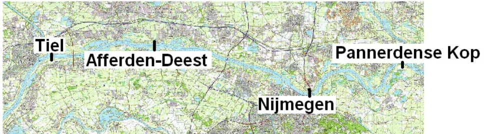
Because rivers are not usually rectangles, it is more difficult to give a realistic presentation of the boundaries of the river with a rectangular grid. In the curvilinear grid, the natural boundary of the river usually coincides with the grid points so no inaccuracies at the boundary are introduced [Warmink, 2009]. Therefore, a curvilinear grid is usually less inaccurate than a rectangular grid and is regularly used for rivers. WAQUA [Rijkswaterstaat, 2012] and Delft3D [Deltares, 2014] are based on the curvilinear grid. However, some drawbacks of curvilinear grids cannot be easily circumvented. Staircase representation of closed boundaries is sometimes unavoidable and in the inner bends of meandering rivers, gridlines are focussed, leading to unnecessarily small grid cells [Kernkamp et al., 2011]. Figure 2 shows an example of staircase representation at Nijmegen, where the summer bed is narrowed. As a result, the grid cells of the curvilinear WAQUA grid are not following the quay wall at Nijmegen well, although the flow velocities can be quite large.

Increasingly more models use a triangular grid, like Telemac [EDF-R&D, 2013] and MIKE 21 [DHI, 2011]. The advantage of a triangular grid is that it is more flexible in the representation of the mesh, because the mesh can be locally refined. However, the unstructured grid requires another numerical solution method. According to [Garcia, 2008], the grid refinement flexibility is obtained at the price of computational efficiency, because the used numerical method for the structured grid is computational more efficient.

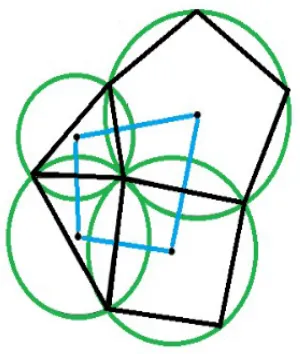
Flexible Mesh combines the curvilinear grid and the triangular grid of both models. For computational efficiency curvilinear grids aligned with the main flow direction in the river are favoured [Kernkamp et al., 2011]. Triangular grids can then be used to refine the grid locally in complex locations to maintain high accuracy. Figure 3 shows an example of the application of grid refinement and alignment of the Waal river in a bend, using triangles. For computational efficiency, the unstructured grid in Flexible Mesh also needs to be orthogonal. The orthogonality of common faces of adjacent grid cells with the lines connecting the centres of the adjacent cells imposes two requirements [Verwey et al., 2011]:

1. The corners of two adjacent cells are positioned on a common circle. 2. The centre of each cells falls within its boundaries.

Figure 4 shows an unstructured grid example of the principle of orthogonality. All corners are positioned on a common (green) circle and the centre of the cell, connected with the blue lines, falls within its boundary.

1.3 Numerical solution

As described in previous section, unstructured grids require another numerical solution method as structured grids. Some fundamental differences between the numerical solution methods for structured and unstructured grids will be discussed in this section.

The hydrodynamic models WAQUA and Delft3D use a curvilinear grid. The space derivatives of the shallow water equations are computed using finite difference method (FDM) for a staggered grid. In WAQUA, the space discretization is considered by means of central and upwind differences at the points where the unknown variable to be calculated is defined [Rijkswaterstaat, 2012]. For instance, the central difference (equation 5) and the forward difference (equation 6) for at the u-velocity point (cell m, n) is given by:

δ

u

δ ζ

=

u

−

u

2

δ

u

δ ζ

=

u

−

u

By combining both central and the first order upwind scheme a second order upwind scheme is proposed (equation 7 and equation 8). The advantage of a second order scheme is that it is more accurate than a first order scheme, as the error is of a higher order.

δ

u

δ ζ

=

1

2

(−

3u

+

4u

−

u

)

δ

u

δ ζ

=

1

2

(

3u

−

4u

+

u

)

The time derivatives of the shallow water equations are computed by using an Alternating Direction Implicit

(ADI), which is a FDM in which the variables are arranged in a staggered grid. The water level disturbance ζ and the flow velocities u and v by a time advancement procedure in which the integration proceeds in increments of half time steps [Rijkswaterstaat, 2013]. In the first step v is calculated separately from u and ζ and in the second step u is calculated separately from v and ζ. So the finite differences equations, derived from the Taylor series expansion, are split into two. One equation is taken implicitly with the x-derivative and one equation is taken implicitly with the y-derivative. According to [Rijkswaterstaat, 2013], this approach has the advantage that it is computational efficient and, although the accuracy puts a limit on the time step, it is unconditionally stable. The FDM cannot be applied for models based on unstructured grids.

To solve numerical problems for unstructured grids, the finite element method (FEM) and the finite volume method (FVM) can be used. Telemac is an example of a 2D hydrodynamic model which uses a triangular grid and the finite element method (FEM) as solution method. FEM is very flexible for the representation of complicated geometrics, for example a triangular shape [Vreugdenhil, 1994]. The values of the unknowns h (water level), u (streamwise velocity) and v (lateral velocity) are computed at the nodes (corners of triangular) of each element. The values within the elements (non-nodal points) are approximated by piecewise polynomial interpolation. The values in the elements are interpolated by using the values at the nodes of the element and trial functions. The trial functions are predefined and approximate the variation within an element. Because the trial functions generate an error compared to the differential equations since the trial function does not guarantee conservation of mass, the equations are not yet satisfied. The residual, the error caused by the trial function, is distributed by weighted functions in order to approximate the differential equations. The analytical equations for the different elements can be rewritten to numerical equations for the numerical solution. The limitation of the FEM can be that a solution or physical data might vary rapidly compared to the distance between nodes, leading to inaccuracies. However, refining the grid can improve the accuracy, but also needs more modelling effort.

Flexible Mesh uses the FVM as numerical solution. The FVM is based on discretization of the integral form of the conservation equations, where the FDM is based on the differential form of the conservation equations. The FVM guarantees conservation of mass and momentum. As in WAQUA, a staggered grid is used for the numerical solution in Flexible Mesh. Time integration of the shallow water equations is done using the implicit θ-method. Only the advection term in the momentum equation is integrated explicitly. In Flexible Mesh, the equations are solved in a combined solver. A part of the water level unknowns is solved directly by Gaussian elimination and the remaining unknowns are solved by the iterative conjugate gradients (CG) solver. [Kernkamp et al., 2011] The advantage of using Gaussian elimination is that the more time consuming CG solver is needed for less unknowns. However, the Gaussian elimination can only be used until a maximal degree of unknowns is reached. According to [Verwey et al., 2011], in most cases more than 50% of the equations is solved by Gaussian elimination.

1.4 Differences numerical solution

An important difference between the FEM and FVM and the FDM is that the integral form of the shallow water equations are better suited than the differential form to deal with complex geometries in multi-dimensional problems as the integral formulations do not rely in any special mesh structure [Peiró & Sherwin]. Therefore, the FDM is not suitable to be applied for an unstructured grid. Further, the functions of the FDM are bound to the grid which makes the FEM and FVM easier to analyze [Gunzburger & Peterson, 2013]. The advantage of FDM is that the method more computational efficient for a given network size than the FEM and FVM. However, the FME and FVM method are better able to accommodate irregular shapes and therefore FDM often require finer grids. Further, in Flexible Mesh triangular cells can be combined with curvilinear grids. The computational efficiency in Flexible Mesh can be improved by limiting the use of triangular cells and using curvilinear cells aligned with the flow direction [Kernkamp et al., 2011].

As described in previous paragraph, the FDM method in WAQUA is unconditionally stable which allows a larger time step. Flexible Mesh integrates the advection term explicitly and is restricted by the Courant number. The condition is expressed by the Courant-Friedrichs-Lewy condition (CFL condition). The CFL condition is given by equation 9, in which c is the wave celerity. In Flexible Mesh, the default maximum value for the CFL condition is 0,7 [Van Dam et al., 2014]. Because this condition is applied for the whole grid, the smallest grid cell is normative for the CFL condition. Therefore, the time may be decreased because of a local grid refinement. During the simulation Flexible Mesh automatically adapt the time step based on the CFL condition.

(

c

+

u

)

δ

t

Where c is the celerity of the flood wave and dt/dx represents the ratio between the used time step in the model and the length of a grid cell.

Studies for the different methods and models state that there is not one best numerical solution method. Studies with the model with the unstructured grid in development showed the same order of accuracy as WAQUA and Delft3D, models with a curvilinear grid which are known as efficient shallow-water models [Kernkamp et al., 2011]; [Verwey et al., 2011]. However, in the study of [Kernkamp et al., 2011], it was shown that the computational time of the Flexible Mesh model was in the same order but still longer than for WAQUA and Delft3D. The results showed potential for further development of the unstructured grid.

1.5 Research objectives

Flexible Mesh is a new model which is significantly different from commonly in The Netherlands used models WAQUA and Delft3d. While Flexible Mesh is still under development, the model needs to be tested and validated for specific cases. In this research Flexible Mesh is tested and compared with the structured grid based WAQUA and the possibilities of the unstructured mesh of Flexible Mesh are applied on a side channel at Afferden at Deest where the WAQUA grid is considered to be inaccurate. The main objective of this research is:

Evaluate the performance (water levels, flow velocities and discharges) of Flexible Mesh by comparing with WAQUA and assess the sensitivity of the modelling results for the grid resolution in Flexible Mesh.

The model results of Flexible Mesh should be compared to the model results of WAQUA as the project Afferden-Deest is originally modelled in WAQUA. Important hydrodynamic parameters such as the water levels, flow velocities and the discharge distribution over the Waal and the side channel will be used for the evaluation. In order to make a good comparison between the results in WAQUA and Flexible Mesh, first processes which might cause differences will be analyzed. As a result, the following research questions are formulated and serve as a guideline for this report:

1. Which processes in the Flexible Mesh model and WAQUA model cause differences between both models?

2. What are the differences in the results of the water levels, flow velocities and discharges between WAQUA and Flexible Mesh for the testcase without side channel and with side channel?

3. What is the effect of increasing the grid resolution in Flexible Mesh on the results of the water levels, flow velocities and discharges?

The first two research questions focuses on a comparison between WAQUA and Flexible Mesh by using the same schematization. The third research question focuses on the application of local grid refinements in Flexible Mesh. Goal of the local grid refinement is to assess if the accuracy of the schematization might be increased by increasing the grid resolution.

1.6 Case Afferden-Deest

width of circa 100 meter.

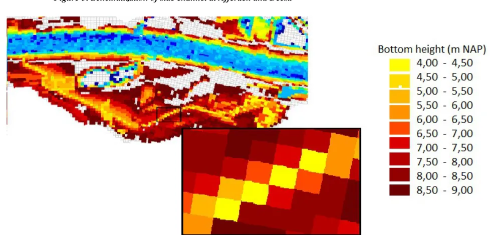
In order to predict the impact of the side channel, the side channel is modelled in WAQUA with a usual curvilinear grid. Figure 5 shows a schematization of the side channel at Afferden and Deest. However, compared to the main channel of the Waal, the side channel is not straight and the channel is relative small. Because of the geometry of the side channel, the variations in the side channel are quite large compared to the variations in the Waal. The width of the side channel is less than 100 meter for the largest part of the side channel while the grid cells of the WAQUA grid have a size of 40x30 meter. So the geometry of the side channel is in the model just schematized by a few grid cells over the width. Therefore, there are concerns about the accuracy of the schematization of the WAQUA model. Figure 6 shows the geometry of the side channel projected on the WAQUA grid. From that figure it can be seen that the variations in bed height between adjacent cells in the side channel is sometimes about 3 meter. Further, locally the side channel is just presented by two grid cells over the width. Staircase representation is also visible in the side channel. The water cannot flow from cell to cell via the corner. Therefore, the water in the side channel will not flow in a straight line but will follow the 'stairs'. Because of the height differences between the cells the staircase representation will probably be obstructive for the flow.

Figure 5: Schematization of side channel at Afferden and Deest.

In order to improve the representation of the side channel, the resolution of the grid in the side channel needs to be increased. Further, the staircase representation of the side channel can be avoided by aligning the cells on the flow direction of the side channel. For this case, the possibilities of the unstructured grid of Flexible Mesh seem to be suitable to improve the schematization. Results in the model of the water levels, flow velocities and discharges through the side channel and Waal main channel are of special interest.

1.7 Thesis outline

In chapter 2 the methodology for the analysis of differences between WAQUA and Flexible Mesh will be described. Subsequently, the results of the analysis for two testmodels are discussed (Research question 1). In chapter 3 the methodology for the comparison between WAQUA and Flexible Mesh and for the grid refinement, which will be partly based on the results in chapter 2, is described. In chapter 4 the results of the comparison between WAQUA and Flexible Mesh for the Waal (research question 2) will be discussed followed by the results of the grid refinement in Flexible Mesh (research question 3). In chapter 5 the model results of Flexible Mesh and the limitations of this research will be discussed. Finally the conclusions and recommendations are presented in chapter 6.

In this study different simulations in Flexible Mesh and WAQUA are executed in order to answer the research questions. Table 1 gives an overview of the different modelling runs executed in this study and the purpose of the modelling runs.

Table 1: Overview of modelling runs executed in this study.

Computation

Goal of computation

Section

Testmodels

Analyze differences between FM and WAQUA

2.2 + 2.3

Waalmodel (without and with

side channel)

Compare model results between FM and calibrated

WAQUA model

4.1

Local grid refinement

Assess effect of local grid refinement at Afferdense and

2 Analysis differences WAQUA – Flexible Mesh

Before working on model simulations for the testcase, first the WAQUA and Flexible Mesh models are analyzed for basic model cases. The goal of this analysis is to observe which processes may cause large difference between WAQUA and Flexible Mesh. Besides it will give a better understanding of the model, this analysis will be used to choose appropriate input for the other parts of the research. First, an outline of important differences in model settings between WAQUA and Flexible Mesh will be given which might cause differences in the results. Then the method for this analysis will be described. Finally results will be shown for a basic case and a more realistic case of a part of the Waal. Table 2 gives an overview of the different modelling runs of testmodels executed in chapter 2 and the purpose of the modelling runs.

Table 2: Overview of testmodels executed in chapter 2.

Computation

Goal of computation

Section

Rectangular testmodel

Analyze differences between FM, WAQUA and

analytical estimation for model with uniform roughness

2.2

Testmodel Waal

(uniform roughness)

Analyze differences between FM and WAQUA for

model with uniform roughness

2.3

Testmodel Waal

(spatial variable roughness)

Analyze differences between FM and WAQUA for

model roughness defined with trachytopes

2.3

2.1 Model differences WAQUA – Flexible Mesh

Flexible Mesh has some default model settings which are significantly different from the assumptions in WAQUA. These assumptions might cause differences between WAQUA and Flexible Mesh while the schematization of the model is the same. The differences that are already known are described shortly.

2.1.1 Colebrook-White formula

The first difference between WAQUA and Flexible Mesh is the used Colebrook-White formula. The used Colebrook-White formula in Flexible Mesh has added a correction to the formula used in WAQUA to improve the representation of the hydraulic radius. This formula results in a 7 to 8 % higher bed friction in Flexible Mesh. The used formulas in WAQUA and Flexible Mesh are presented in respectively equation 10 and 11 [Van Der Pijl, 2013].

1

√

C

=

1

κ

ln

(

h

e min

(

1

30

K

,0.3

h

)

)

1

√

C

=

A

κ

ln

(

h

2.5

min

(

1

30

K

,

h

15

)

)

, A

=

18

κ

√

g

ln

(

10

)

≈

1.0233

2.1.2 Conveyance

The second difference is the default setting in Flexible Mesh to represent the bottom height within a grid cell. In WAQUA the bottom level within a grid cell is always constant, so the bed is schematized as a horizontal tile. In Flexible Mesh the default setting enables to represent the bottom level in a cell by a diagonal tile between two bed level points. Especially in complex areas with relative large bed level variations, the representation in WAQUA may lead to inaccuracies in the water depth within a grid cell. Further, there is a height difference between the bed of two adjacent grid cells in the WAQUA model because the bed level in the WAQUA model does not represent the real bed level at the bed level point. Therefore, there will be inaccuracies in the calculation of the equilibrium water depth. Because in Flexible Mesh the bed level may vary between two bed level points, the real bed level can be used at the bed level points. (Figure 7) In Flexible Mesh there is also an option to disable the Conveyance2D setting and represent the bottom of a cell as a horizontal tile. This option will be used to assess the effect of representing the bed within a grid cell with a constant level or with a varying height.

2.1.3 Energy losses by weirs

The third difference is the modelling of energy losses by flow over weirs. In WAQUA the energy losses are directly added to the momentum equation as an opposing force by adding a term -gΔE/Δx to the right hand side of the momentum equation [Rijkswaterstaat, 2012]. In Flexible Mesh a subgrid formulation is used for the energy losses. Upstream of the weir there is calculated with conservation of energy and downstream of the weir there is calculated with conservation of momentum. Further, the formula for the calculation of the energy height is not the same in WAQUA and Flexible Mesh. As there are many weirs in the Dutch rivers (e.g. groynes) the effect of weirs can be large. Therefore, model results with and without weirs will be obtained to assess the effect of weirs in WAQUA and Flexible Mesh.

2.1.4 Thin dams

In the schematization of a river many points where no water can flow are represented by thin dams. An example for a thin dam might be a structure (e.g. bridge pillars), which affects the flow in a river. Because the numerical method of WAQUA and Flexible Mesh is different, the effect of thin dams on the model results might be different. The effect of thin dams on the model results in Flexible Mesh and WAQUA will be tested.

2.2 Rectangular testmodel

2.2.1 Method

First a small rectangular model is considered. This schematization is a very elementary schematization in which a rectangular grid of 2000x200 meter with grid cells of 40x40 meter is schematized. Therefore, the grid contains 5 cells over the x-direction (m=6) and 50 cells over the y-direction (n=51). A constant discharge

of 1515 m3/s is considered at the inflow boundary and a constant water level of 11.70 meter is considered at the outflow boundary of the grid. The bed is horizontal (slope is 0.00 m/m) at a level of 5.00 meter. Between 400 and 480 meter from the inflow boundary of the grid, there is a sill at a level of 5.30 meter. (Figure 8)

The model is schematized in WAQUA and converted from WAQUA to Delft3D by the MatLab tool ‘Simona2mdf’ and converted from Delft3D to Flexible Mesh by the MatLab tool ‘dflowfmConverter.m’, which are available in the OpenEarthTools [Deltares, 2014a]. a uniform Colebrook-White roughness is used (Ks = 0.20).

In first instance, the default settings are used in the WAQUA model and the Flexible Mesh models. Because of the low complexity of the model, small differences are expected between both models. Because of the low complexity it is also possible to verify the results with analytical approximations. For the analytical approximation the law of Chézy is used (equation 12):

u

=

C

_√

(

hi

)

Q

hB

=

C

√

(

hi

)

Because the used Colebrook-White formula is different in WAQUA and Flexible Mesh, for both models a different water level is approximated. At the outflow boundary the water level is known which is 11.70 meter. The bed level is at 5.00 meter so the water depth is 6.70 meter. The Chézy roughness can be calculated with the formula of Colebrook-White (equation 10 and 11) and using equation 13.

C

=

g

C

Flexible Mesh model default uses another formula for the Colebrook-White roughness than WAQUA. To assess the effect of the used formula the Flexible Mesh model is simulated with the Flexible Mesh formulation and WAQUA formulation of the Colebrook-White formula. Therefore, the following results are obtained:

– Two analytical approximations (WAQUA and Flexible Mesh formulation of Colebrook-White formula)

– Simulation of WAQUA model

– Two simulations of Flexible Mesh model (WAQUA and Flexible Mesh formulation of Colebrook-White formula)

2.2.2 Results

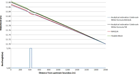
The water level of the models for WAQUA and Flexible Mesh are shown in Figure 9. Also the analytical calculated water level is shown in the figure for the Colebrook-White formula formulated by WAQUA and Flexible Mesh.

From the results it can be seen that the difference between WAQUA and Flexible Mesh is about 1 centimeter, which is quite large for a simple model with a length of just 2 kilometers. However, the results of the WAQUA model and Flexible Mesh model agree quite well with the analytical estimation.

In Figure 10 the water levels of the analytical estimation and the WAQUA and Flexible Mesh model with the Colebrook-White formula of WAQUA are presented. When the same Colebrook-White formula is used the water levels of WAQUA and Flexible Mesh coincide exactly to each other. As expected for this simple model, the modelled water levels of WAQUA and Flexible Mesh do not differ except from the influence of the Colebrook-White formula.

2.3 Testmodel Waal

2.3.1 Method

The Flexible Mesh model behaves like expected for the rectangular model. In this section the model will be tested for a part of the river Waal, which is part of the Rhinemodel. The schematization is shortened such that about 40 km of the Waal is considered downstream of the Pannerdense Kop (from km 884 until km 923). The river reach is considered from Nijmegen (Figure 11). The boundary conditions are obtained from the original Rhinemodel. The inflow is constant 10074 m3_{/s in the Waal, based on the 16.000 m}3_{/s design} discharge at Lobith. The water level at the downstream side of the considered part of the Waal is constant 10.38 meter. As initial conditions, the modelling results of the original Rhinemodel are assumed. The Flexible Mesh model is obtained by using the same converters in the OpenEarthTools as used for the rectangular test model.

Figure 11: Schematization of considered part of the Waal in testmodel.

At first instance the WAQUA and Flexible Mesh model are simulated with the default settings. After the results of WAQUA and Flexible Mesh were known, the impact of certain settings are analyzed. For each simulation one setting in the Flexible Mesh model is changed. The impact on the difference between the WAQUA model and the Flexible Mesh model for a certain setting is obtained by determining the difference with the models with the default settings. Further, settings with a relative large effect on the difference between WAQUA and Flexible Mesh are changed in one simulation in order to assess if the changed settings explains the difference in water level between WAQUA and Flexible Mesh well.

The impact on the difference between WAQUA and Flexible Mesh of settings that are investigated with the following cases:

1. The impact of energy losses by weirs; weirs are deleted from the WAQUA and Flexible Mesh model. 2. The impact of dry cells (thin dams); thin dams are deleted from the WAQUA and Flexible Mesh

model.

3. The conveyance setting; conveyance setting of WAQUA used in Flexible Mesh.

4. The Colebrook-White formula; Colebrook-White formula of WAQUA used in Flexible Mesh. 5. Cases with large effect on differences between WAQUA and Flexible Mesh combined.

In first instance the roughness in the schematization is defined with a uniform Colebrook-White roughness (Ks = 0.20) as in the rectangular testmodel. After the differences are obtained for the testmodel of the Waal with the uniform Colebrook-White roughness, the roughness in the WAQUA and Flexible Mesh model is defined with trachytopes. By using trachytope files the roughness can be defined for all grid cells separately, so for example roughness by vegetation can be described with trachytope files. The trachytope files were already available in the WAQUA model. The trachytope files for Flexible Mesh are obtained by using the available trachytope converter in the OpenEarthTools [Deltares, 2014a].

2.3.2 Results

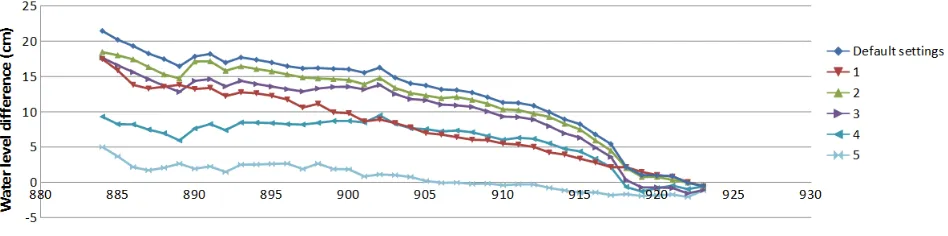
The impact of different settings in WAQUA and Flexible Mesh are obtained for a part of the Waal with a constant Colebrook-White roughness and with a roughness defined by trachytopes. In Figure 12 the difference between the water level in WAQUA and Flexible Mesh is presented as function of the location along the Waal. The six lines in the figure are explained in Table 3. The impact of the settings in Figure 12 and Figure 13 are not exactly representative for the differences of the setting in WAQUA and Flexible Mesh, because another Colebrook-White formula is used so the roughness is different in WAQUA and Flexible Mesh. However, the results are a good indication of the impact of the differences between WAQUA and Flexible Mesh.

Table 3: Investigated settings for the 6 cases for the Waal to analyze differences between WAQUA and Flexible Mesh.

Case

Investigated setting

Default settings

Reference case

1

Weirs deleted from WAQUA and Flexible Mesh model

2

Dry points deleted from WAQUA and Flexible Mesh model

3

WAQUA conveyance setting used in WAQUA and Flexible Mesh

4

WAQUA Colebrook-White formula used in WAQUA and Flexible Mesh

The differences between the WAQUA model and the Flexible Mesh model with default settings are larger than 20 centimeters at the upstream boundary. From the changed settings, using the WAQUA form of the Colebrook-White has the largest impact. The difference between WAQUA and Flexible Mesh is more than halved. Further the difference has decreased with about 5-10 centimeters when the weirs are deleted from the WAQUA and Flexible Mesh model. Using the WAQUA setting for the conveyance decreases the difference with about 5 centimeter while the effect of deleting the dry points in the models is a few centimeters. When case 1, 3 and 4 are combined the differences between WAQUA and Flexible Mesh are smaller than five centimeters at all locations along the Waal.

Subsequently the same analysis is done for the Waal testmodel with trachytopes defining the bed roughness. The different cases which are investigated are explained in Table 3. The difference between the water level in WAQUA and Flexible Mesh is presented as function of the location along the Waal in Figure 13.

The difference for the Waal testmodel with trachytopes used for the bed roughness has a maximum difference of almost 40 centimeter between Flexible Mesh and WAQUA. The difference is in the range of the 95% confidence interval of the design water levels in the Waal for the roughness, found by [Warmink et al., 2013], which is significant in Dutch river management. The differences are higher than for the schematization with the uniform Colebrook-White roughness. However, the absolute impact of the different settings are comparable to the schematization with the uniform Colebrook-White roughness. The result of that simulation with the first, third and fourth case combined, shows that the difference between WAQUA and Flexible Mesh is for the whole Waal smaller than three centimeter. Only at the upstream boundary the water level difference is larger. The difference at the upstream boundary is probably caused by a different approach for solving inflowing water. Overall, the results of the model of the Waal are quite reasonable as the differences can be explained by operational causes.

Figure 13: Water level difference Flexible Mesh - WAQUA for the Waal (km 884-923) for model with trachytopes.

2.4 Conclusions testmodels

For the simulated test models quite large differences are observed between the water levels in WAQUA and Flexible Mesh. For the schematization of the Waal with a uniform Colebrook-White roughness, the maximal difference is almost 25 centimeters, while for the schematization with trachytopes, used to define a spatial variable roughness, the maximal difference is almost 40 centimeters. Based on the observed differences between WAQUA and Flexible Mesh, the much higher water levels in Flexible Mesh seem to be caused by operational differences. The different formula for Colebrook-White in Flexible Mesh compared to the formula in WAQUA results in the largest part of the differences between WAQUA and Flexible Mesh. Further the setting of the conveyance in Flexible Mesh is responsible for a difference of about 5 centimeter. The energy losses by weirs are computed differently in Flexible Mesh and WAQUA, causes a difference of about 10 centimeter. If the WAQUA setting is used for the conveyance and for the Colebrook-White formula and the weirs are neglected in both models, the difference is close to 0 centimeter. Therefore, Flexible Mesh appears to give comparable results to WAQUA besides the mentioned operational differences. In the introduction it was described that WAQUA and Flexible Mesh use different numerical solution methods, which might cause differences in the results. However, from the results it seems that the numerical performance of both models is quite similar.

For the comparison between WAQUA and Flexible Mesh, a choice has to be made for the model settings in Flexible Mesh. For the comparison with WAQUA it is desired to use the same input data in Flexible Mesh. The Colebrook-White formula in Flexible Mesh is responsible for a large difference for the water levels with WAQUA. The Colebrook-White formula is connected to the (friction) input and the formula is not directly influencing the numerics of the Flexible Mesh model. Therefore, for the comparison of Flexible Mesh with WAQUA the Colebrook-White formula of WAQUA is used in Flexible Mesh.

3 Methodology of comparison and grid refinement

In the previous chapter the differences between WAQUA and Flexible Mesh are analyzed. From the simulated testcases a better understanding is obtained from the Flexible Mesh model. The following step is the comparison between modelling results of WAQUA and Flexible Mesh for the case study (research question 2). For the comparison a calibrated WAQUA model will be used which schematizes a real situation. The comparison is done for the Waal with and without side channel at Afferden and Deest. The second step is the application of grid refinement to the side channel at Afferden and Deest (research question 3). In this chapter, the research method for both steps will be described.

3.1 Comparison Flexible Mesh – WAQUA

The comparison between Flexible Mesh and WAQUA is done for the Waal with special focus on the Afferdense and Deestse Waarden. For the Waal without side channel, a Rhinemodel in WAQUA is available which is calibrated based on the high water in 1995. There are also water level measurements available for 1995. For the Waal with side channel, a Rhinemodel is available in which several measures are implemented, including the side channel at Afferden and Deest. Both cases will be described in this section.

3.1.1 Waal without side channel

The calibrated WAQUA model is available for this case. The input of the WAQUA model of the Rhine, which was delivered by Rijkswaterstaat Oost-Nederland, is used as well in Flexible Mesh for a comparison between both models. Because the scale of the Rhinemodel is much larger than the study area, the schematization is shortened to about a 50 km reach of the Waal from de Pannerdense Kop to a few kilometers after Tiel (km 870 to km 919). (see Figure 14 for the schematization of the case study) In this reach there are two measurement locations, at Nijmegen haven and at Tiel. For these locations measurements of water levels are available, which are delivered by Rijkswaterstaat Oost-Nederland to Deltares for the benefit of the calibration and verification of the 1995 Rhinemodel. The downstream boundary condition of the Waalmodel is determined based on the output of the Rhinemodel. A few kilometers downstream from Tiel a Qh-relation is defined. Because the downstream boundary is close to Tiel, the model results are affected by the Qh-relation. Therefore the measurements at Tiel will not be used.

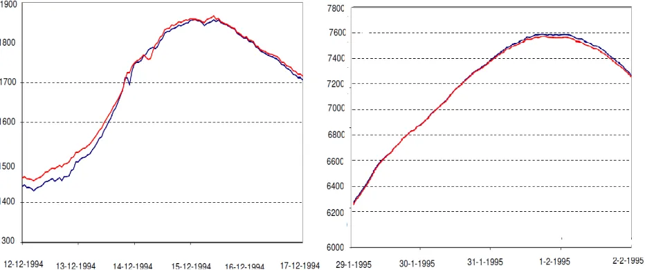
The WAQUA model is calibrated for a high water situation (1995) and for low discharges (1994) as well. Both situations are used for the comparison of the models. A large difference between both discharge regimes is that at low discharge, the flow is going mainly through main channel and at high discharge the flow also going over the floodplain. The low discharge period reaches its peak at 15 December. The high water situation reaches its peak at 1 February 1995. (Figure 15) Two discharges are given for the Waal. In first instance, the discharge was estimated based on measurements. Later a correction to the estimated

discharge was made to improve the estimated discharge for the calibration of the WAQUA model. The discharge after correction is used for this study.

The WAQUA model is again converted to Flexible Mesh with the OpenEarthTools. In Flexible Mesh, the same input data is used as in WAQUA. The default setting of the Colebrook-White formula is changed to the WAQUA formula for Colebrook-White, as explained in section 2.4.

For the Waal without side channel the water levels at the measurement locations Nijmegen haven are mainly used to compare the models. The water levels in Flexible Mesh can be compared to the water levels in WAQUA and the measured water levels in 1994 and 1995. Because Flexible Mesh has the same input as the WAQUA model and the WAQUA model is calibrated for those discharges, the water levels in Flexible Mesh should be close to the water levels in WAQUA.

3.1.2 Waal with side channel

For the Waalmodel with side channel a WAQUA model is available in which measures, including the side channel at Afferden and Deest, are added. This schematization cannot be compared to the calibrated Rhinemodel for 1995, because besides the side channel at Afferden and Deest many other measures are added (e.g. side channel at Lent). Therefore, the downstream boundary condition (Qh-relation) is determined again based on the results of the Rhinemodel with the side channel. Further, the models are obtained in the same manner as the Waalmodel without side channel. The converters in OpenEarthTools are used to obtain the schematization in Flexible Mesh.

Although in reality it will be a permanently flowing side channel, with the schematization no discharge is flowing through the side channel at low discharges. Therefore, the Waal with side channel is only simulated for the high discharge in 1995. Because the schematization represents a not yet existing situation, measurements cannot be used to compare with model results. However, the schematization consists of the side channel at Afferden and Deest which is interesting for a comparison of model results of WAQUA and Flexible Mesh. For the side channel it is interesting what effect the side channel has on the water levels locally in WAQUA and Flexible Mesh. Further, the difference in flow velocities in the side channel and the discharges through the side channel and main channel of the Waal are compared between the WAQUA results and the Flexible Mesh results.

3.2 Grid refinement

Local grid refinement is applied to the case project Afferden-Deest to assess the impact on the results of the Flexible Mesh model. The grid refinement is applied to the main channel of the Waal next to the side channel at Afferden and Deest and to the side channel at Afferden and Deest itself. First, the setup of the model for the grid refinement is explained.

3.2.1 Model setup

For the study of the local grid refinement as reference situation the same schematization of the Waal with side channel is used as for the comparison of WAQUA and Flexible Mesh. The high discharge of 1995 is considered for the model. The use of the trachytope files to define the roughness is not yet supported for the unstructured grid in Flexible Mesh. However, to assess the effect of local grid refinement the same model settings are needed for different simulations. Therefore the output of the roughness from the Flexible Mesh model with the original schematization is used as input for the simulations in the study of local grid refinements. The Colebrook-White values for all network links at the peak of the discharge wave are exported. The netlinks in the file are written to x- and y-coordinates such that the file can be used as input file. In the schematization all default settings of Flexible Mesh are used. So in this schematization the default Colebrook-White formula for Flexible Mesh is used.

For the reference schematization the input data is projected on the network of Flexible Mesh. When the grid is adapted the input data is not any more defined on the network. Therefore, when the grid is refined the input data (roughness and bathymetry) is newly projected to the adapted part of the network. The data is interpolated to the network links of the grid.

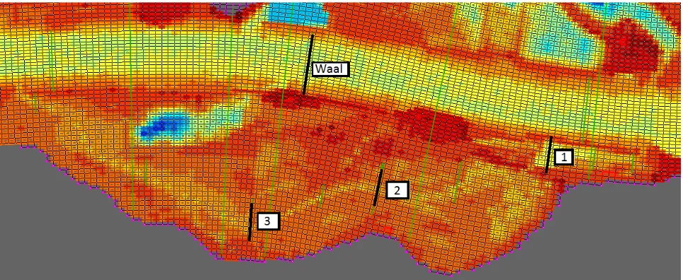
Changes of the flow in a river may have large influences on the long term for a river. Therefore, specific information about the discharge at the side channel at Afferden and Deest is desired to evaluate the impact of grid refinement. Some cross sections are added to the schematization to observe the discharge in the side channel and in the main channel. In Figure 16 the cross sections, one in the main channel of the Waal and three in de side channel, are presented with black lines. These three cross sections for the side channel are drawn perpendicular to the side channel. Therefore, the cross sections also fit for the aligned side channel.

3.2.2 Grid refinement main channel

First, the grid refinement is applied to the main channel of the Waal over the length of 4 kilometer next to the side channel at Afferden and Deest. The refinement of the Waal channel is used as reference situation for the refinement of the side channel. The variations between adjacent grid cells are much larger in the side channel than in the main channel of the Waal. Therefore, the expectation is that the WAQUA grid is quite accurate for the main channel of the Waal, but is inaccurate for the side channel at Afferden and Deest. The refinement of the Waal channel is used to check if the effect of refining the grid of the side channel is indeed larger than refining the grid of the Waal channel.

The grid of the main channel of the Waal is refined over the width, so the length of the cells remains the same but the number of cells over the width of the Waal channel increases. In Flexible Mesh, this grid refinement is executed automatically by defining the grid to be refined with a polygon. The cells are refined by using the Casulli-type mesh refinement. After the automatical refinement the quality of the grid is monitored and improved where needed. Particularly at the boundary of the refinement, where the transition from the original grid to the refined grid is, the mesh quality might have some trouble with the orthogonality. The model is simulated with the WAQUA grid and with the grid resolution two, four and eight times increased compared to the reference situation. Because the impact of the grid refinement in the Waal channel is expected to be limited, the model results are probably not much affected by higher grid resolutions.

3.2.3 Grid refinement side channel (not aligned)

The grid refinement for the side channel is executed with help of the bathymetry data. The refined part of the grid includes the parts of the side channel in which the variation in bed level between adjacent grid cells is relative large. The refinement is extended from the inlet to the outlet channel of the side channel. A with the flow direction aligned grid is assumed to be computational more efficient. Therefore, the grid refinement in the side channel is applied with an aligned and not aligned grid refinement.

The grid refinement is, just as for the refinement of the main channel of the Waal, executed over the width of the side channel, so the length of the grid cells remains the same. The grid refinement without alignment is executed by defining a polygon and applying the Casulli-type refinement on the original WAQUA grid which refines the grid within the polygon two times.

3.2.4 Grid refinement side channel (aligned)

For the evaluation of the grid refinement the discharge, flow velocities and water levels are used as model results. The discharges and flow velocities are observed in the side channel and the main channel of the Waal. The water levels are observed just before the inlet channel of the Waal, where the impact of the side channel on the water level is largest. An important evaluation criteria for the grid refinement is whether convergence of the model results is observed or not. It is expected that the influence of grid refinement will decrease when applying on a higher grid resolution. The Waalmodel is simulated with a refinement of the side channel of two, four and eight times. So including the original grid, four simulations are executed. It is expected that convergence can be seen after at least three refinements. Additional, the performances of the model will be observed. Because the minimal cell size is decreasing after the refinements, the time step might need to be decreased to meet the CFL criteria. As a result the calculation time will increase. Therefore, the simulation time of the models with the side channel refinement are evaluated.

4 Results

In this chapter the results of the research are presented. First the results of the comparison between WAQUA and Flexible Mesh will be described (research question 2). The comparison consists of a schematization without side channel for which measurements are available and a schematization with side channel. Secondly the results of the local grid refinement at Afferden and Deest will be presented (research question 3). The local grid refinement is divided in a refinement of the main channel of the Waal and a refinement of the side channel. Table 4 gives an overview of the different modelling runs executed in chapter 4 and the purpose of the modelling runs.

Table 4: Overview of testmodels executed in chapter 2.

Computation

Goal of computation

Section

Waalmodel without side

channel

Compare model results of FM with calibrated WAQUA

model and measurements for the Waal

4.1.1

Waalmodel with side channel Compare model results of FM with WAQUA for the case

study Afferden and Deest

4.1.2

Local grid refinement in main

channel of Waal

Assess effect of local grid refinement in main channel of

Waal as reference case

4.2.1

Local grid refinement in side

channel without alignment

Assess effect of local grid refinement in side channel

without aligning the grid to the flow direction

4.2.2

Local grid refinement in side

cannel with alignment

Assess effect of local grid refinement in side channel

with aligned grid to flow direction

4.2.3

4.1 Comparison Flexible Mesh – WAQUA

This section describes the results for the comparison between Flexible Mesh and WAQUA for the Waal with and without side channel. As described in Chapter 3, for these simulations the Colebrook-White formula of WAQUA is used in Flexible Mesh. Further, the default settings of Flexible Mesh are used.

4.1.1 Waal without side channel

The Waalmodel, obtained from the Rhinemodel, is calibrated for the high discharge wave in 1995 and low discharge wave in 1994. The model is simulated for both discharge waves. Additional to the modelling results of WAQUA and Flexible Mesh, data is available of measurements at Nijmegen haven. The measurements are delivered by Rijkswaterstaat Oost-Nederland to Deltares. In Figure 18 the modelling results of WAQUA and Flexible Mesh and the measured water levels are presented for the high discharge in 1995 and the low discharge in 1994.

For the high discharge wave Flexible Mesh results in higher water levels than WAQUA. At Nijmegen the water level in Flexible Mesh is about 11 centimeter higher than in WAQUA at the peak water level. The difference between WAQUA and Flexible Mesh decreases into the downstream direction, because the Qh-relation on the downstream boundary influences the water levels. For the low discharge wave Flexible Mesh results and WAQUA results do agree very well with each others. A large difference between both discharge regimes is that in the low discharge wave the flow is mainly going through the main channel of the Waal. At high discharges the flow is also going over the floodplain. In the main channel of the river less weirs are present and weirs become mainly important when the flow is going over the summer dike to the floodplain. In chapter 2 it was observed that weirs may have a large impact on the difference between WAQUA and Flexible Mesh. Therefore, the Waalmodel is again simulated but now without weirs in the WAQUA model and the Flexible Mesh model. In Figure 19 it is shown that the difference between WAQUA and Flexible Mesh is about 2 centimeters. The modelling of energy losses by weirs seems to result in higher water levels in Flexible Mesh for high discharges. In Figure 20 the flow velocities at Afferden and Deest are shown at the peak of the flood wave. In the WAQUA model (figures above) the flow velocity in the floodplain is mostly larger than in the floodplain of the Flexible Mesh model (figures below). Therefore, the discharge in the floodplain is larger in the WAQUA model resulting in a lower water level in the WAQUA model compared to the Flexible Mesh model.

The WAQUA model is calibrated such that the water levels at the peak of the flood wave are close to the observed water levels. The Flexible Mesh results deviate 11 centimeter of those water levels for the high

Figure 19: modelled water levels for high discharge in 1995 at Nijmegen haven for schematization without weirs.