http://wrap.warwick.ac.uk
Original citation:Englert, Matthias, Roglin, H., Sponemann, J. and Vocking, B. (2009) Economical
caching. In: 26th International Symposium on Theoretical Aspects of Computer Science, Freiburg, Germany, Feb 2009
Permanent WRAP url:
http://wrap.warwick.ac.uk/47512
Copyright and reuse:
The Warwick Research Archive Portal (WRAP) makes this work of researchers of the University of Warwick available open access under the following conditions.
This article is made available under the Creative Commons Attribution-NoDerivs 3.0 (CC BY-ND 3.0) license and may be reused according to the conditions of the license. For more details see: http://creativecommons.org/licenses/by-nd/3.0/
A note on versions:
The version presented in WRAP is the published version, or, version of record, and may be cited as it appears here.
ECONOMICAL CACHING
MATTHIAS ENGLERT1
AND HEIKO R ¨OGLIN2
AND JACOB SP ¨ONEMANN3
AND BERTHOLD V ¨OCKING4
1 DIMAP and Department of Computer Science, University of Warwick
E-mail address: [email protected]
2
Department of Computer Science, Boston University
E-mail address: [email protected]
3
Institute of Transport Science, RWTH Aachen University
E-mail address: [email protected]
4 Department of Computer Science, RWTH Aachen University
E-mail address: [email protected]
Abstract. We study the management of buffers and storages in environments with un-predictably varying prices in a competitive analysis. In the economical caching problem, there is a storage with a certain capacity. For each time step, an online algorithm is given a price from the interval [1, α], a consumption, and possibly a buying limit. The online algorithm has to decide the amount to purchase from some commodity, knowing the pa-rameterαbut without knowing how the price evolves in the future. The algorithm can purchase at most the buying limit. If it purchases more than the current consumption, then the excess is stored in the storage; otherwise, the gap between consumption and pur-chase must be taken from the storage. The goal is to minimize the total cost. Interesting applications are, for example, stream caching on mobile devices with different classes of service, battery management in micro hybrid cars, and the efficient purchase of resources. First we consider the simple but natural class of algorithms that can informally be described as memoryless. We show that these algorithms cannot achieve a competitive ratio below√α. Then we present a more sophisticated deterministic algorithm achieving a competitive ratio of
1 W(1−α
eα )+1
∈
h√α √
2,
√α+1 √
2
i
,
whereW denotes the Lambert W function. We prove that this algorithm is optimal and that not even randomized online algorithms can achieve a better competitive ratio. On the other hand, we show how to achieve a constant competitive ratio if the storage capacity of the online algorithm exceeds the storage capacity of an optimal offline algorithm by a factor of logα.
1998 ACM Subject Classification: F.1.2, F.2.2.
Key words and phrases: Online Algorithms, Competitive Analysis, Storage Management.
M. Englert is supported by EPSRC grant EP/F043333/1 and DFG grant WE 2842/1. H. R¨oglin is supported by a fellowship of the German Academic Exchange Service (DAAD) and by DFG through German excellence cluster UMIC. J. Sp¨onemann is supported by DFG Research Training Group 1298 (AlgoSyn). B. V¨ocking is supported by DFG through German excellence cluster UMIC.
c
M. Englert, H. R ¨oglin, J. Sp ¨onemann, and B. V ¨ocking
CC
Creative Commons Attribution-NoDerivs License
STACS 2009
1. Introduction
In many environments in which resources with unpredictably varying prices are con-sumed over time, the effective utilization of a storage can decrease the cost significantly. Since decisions have to be made without knowing how the price evolves in the future, storage management can naturally be formulated as an online problem in such environments. In theeconomical caching problem each time step is characterized by a price, a consumption, and a buying limit. In every such time step, an online algorithm has to decide the amount to purchase from some commodity. The algorithm can purchase at most the buying limit. If it purchases more than the current consumption, the excess is stored in a storage of limited capacity; otherwise, the gap between consumption and purchase must be taken from the storage.
This kind of problem does not only arise when purchasing resources like oil or natural gas, but also in other interesting application contexts. Let us illustrate this by two examples, one from the area of mobile communication and one dealing with the energy management in cars. The first example is stream caching on mobile devices with different communication standards like GSM, UMTS, WLAN. Since the price for transmitting data varies between the different standards and since for moving devices it is often unclear which standard will be available in the near future, the problem of cheaply caching a stream can be formulated in our framework. The second example is battery management in micro hybrid cars. In addition to a conventional engine, these cars have an electric motor without driving power that allows the engine to be restarted quickly after it had been turned off during coasting, breaking, or waiting. The power for the electric motor is taken from a battery that must be recharged by the alternator during drive. Since the effectiveness of the conventional engine depends on the current driving situation, the question of when and by how much to recharge the battery can be formulated as an economical caching problem.
Let α denote an upper bound on the price in any step that is known to the online algorithm. Formally, an instance of the economical caching problem is a sequenceσ1σ2. . .
in which every step σi consists of a price βi ∈ [1, α], a consumption vi ≥ 0, and a buying
limit ℓi ≥ vi. During step σi, the algorithm has to decide the amount Bi ∈ [0, ℓi] to
purchase. This amount has to be chosen such that neither the storage load drops below zero nor the storage load exceeds the capacity of the storage, which we can assume to be 1 without loss of generality. Formally, if Li−1 denotes the storage load after step σi−1, then
Bi must be chosen such that Li−1+Bi−vi ∈ [0,1]. The restriction ℓi ≥ vi is necessary
because otherwise covering the consumption might not be possible at all. The economical caching problem without buying limits is the special case in which all buying limits are set to infinity.
1.1. Our Results
First we observe that the following simple algorithm achieves a competitive ratio of√α (this also follows as a special case from Theorem 2.7): In every step σi with price βi ≤√α
buy as much as possible while adhering to the buying limit and the storage capacity. In all other steps buy only as much as necessary to maintain a non-negative storage load.
This algorithm belongs to a more general natural class of algorithms, namely algorithms with fixed buying functions. Given an arbitrary buying function f: [1, α] → [0,1], we can define the following algorithm: For everyσi the amount to purchase is chosen such that the
limit. For example, the buying function f of the simple algorithm satisfies f(x) = 1 for x ≤ √α and f(x) = 0 for x > √α. Informally, algorithms with fixed buying functions can be seen as memoryless and vice versa, in the sense that the action in each step does only depend on the characteristics of that step and the current storage load. However, formally this intuitive view is incorrect since, due to the continuous nature of the problem, an algorithm can encode arbitrary additional information into the storage load. One of our results is a lower bound showing that there is no buying function that gives a better competitive factor than √α.
Our main result, however, shows that this is not the best possible competitive factor. We present a more sophisticated deterministic algorithm that achieves a competitive ratio of
r:= 1
W(1eα−α)+1 ∈ h√
α
√ 2,
√
α+1 √
2
i ,
where W denotes the Lambert W function (i.e., the inverse of f(x) = x·ex). We comple-ment this result by a matching lower bound for randomized algorithms, showing that our algorithm is optimal and that randomization does not help. Our lower bounds hold even for the problem without buying limits.
Finally, we consider resource augmentation for the economical caching problem. We show that, for everyz∈N\{1}, there is a buying function algorithm achieving a competitive ratio of √z
α against an optimal offline algorithm whose storage capacity is by a factor of z−1 smaller than the storage capacity of the online algorithm. In particular, this implies that we obtain a buying function algorithm that ise-competitive against an optimal offline algorithm whose storage capacity is by a factor of max{⌈ln(α)⌉ −1,1} smaller than the storage capacity of the online algorithm.
1.2. Previous Work
Although the economical caching problem is, in our opinion, a very natural problem with applications from various areas, it seems to have not been studied before in a competitive analysis. However, the problem bears some similarities to the one-way-trading problem introduced by El-Yaniv et al. [4]. In this problem, a trader needs to exchange some initial amount of money in some currency (say, dollars) to some other currency (say, euros). In each step, the trader obtains the current exchange rate and has to decide how much dollars to exchange. However, she cannot exchange euros back to dollars. El-Yaniv et al. present a tight bound of Θ(logφ) on the competitive ratio achievable for the one-way-trading problem, whereφdenotes the ratio of the worst possible exchange rate and the best possible exchange rate. Results on variations of one- and two-way-trading can also be found in the book by Borodin and El-Yaniv [1] and in a survey by El-Yaniv [3]. In the two-way-trading problem, the trader can buy and sell in both directions. A related problem is portfolio management, which has been extensively studied (see, e.g., [2, 5, 6]).
for the one-way-trading problem with a fixed target amount and yields a strict competitive ratio of r for that problem.
1.3. Extensions
We can further generalize the economical caching problem. Each step may be charac-terized by a consumption and a monotonically increasingprice function pi(x) : [0, α]→R+,
withpi(α)≥vi. The price function has the following meaning: The algorithm can buy up
to an amount of pi(x) at rate at most x. The problem with a single price βi and a buying
limitℓi for each stepσi is a special case withpi(x) = 0 forx < βi andpi(x) =ℓi forx≥βi.
Such price functions appear, for example, implicitly in the stock market. At any given time, all sell orders for a specific stock in the order book define one price function since for every given pricex there is a certain number of shares available with an ask price of at mostx.
All our results also hold for this more general model. An (online) algorithm can trans-form an instance for the general problem into an instance of the special problem on the fly: A step with consumption vi and price function pi is transformed into a series of steps
as follows: First we determine the maximum rate we have to pay to satisfy the demand as β := inf{x |pi(x) ≥ vi}. Then we generate the following steps (the upper value indicates
the price, the middle value the consumption, and the lower value the buying limit)
1 pi(1) pi(1)
1 +ε pi(1 +ε)−pi(1) pi(1 +ε)−pi(1)
· · ·
β−ε
pi(β−ε)−pi(β−2ε) pi(β−ε)−pi(β−2ε)
β
pi(β)−pi(β−ε) pi(β)−pi(β−ε)
for a small εwith (β−1)/ε∈N. Finally, we append the following steps for the remaining prices
β+ε 0
pi(β+ε)−pi(β)
· · ·
α−ε 0
pi(α−ε)−pi(α−2ε)
α 0
pi(α)−pi(α−ε)
for a small εwith (α−β)/ε∈N.
Ifεis small, this transformation does not change the cost of an optimal offline algorithm significantly and hence, our upper bounds on the competitive ratios still hold.
2. Upper Bound
2.1. The Optimal Offline Algorithm
To describe an optimal offline algorithm it is useful to track the cost-profile of the storage contents. For this, we define a monotonically decreasing function g(x) : [0, α]→[0,1] that is initialized with g(x) := 1 and changes with each step. In the following, we denote the functiong(x) after stepσi by gi(x) and the initial function byg0(x) = 1.
The intuition behindg(x) is that, assuming the storage of the optimal offline algorithm is completely filled after stepσi, a 1−g(x) fraction of the commodity stored in the storage
was bought at pricex or better.
(1) Consumption is satisfied as cheap as possible, i.e., what we remove from the storage is what we bought at the lowest price.
(2) If we have stored something that was bought at a larger than the current price, replace it with commodity bought at the current price. That is, we revoke the decision of the past to buy at the worse price in favor of buying at the current, better price.
Formalizing this yields the following definition
gi(x) :=
(
min{gi−1(x) +vi,1} ifx≤βi,
max{gi−1(x) +vi−ℓi,0} ifx > βi.
Using this definition, we can characterize the cost of an optimal offline algorithm. As described above, consumption is satisfied at the best possible price. This gives rise to the cost incurred in stepσi, namely
Ci :=
Z βi
0
max{gi−1(x) +vi−1,0}dx .
Based on these values, we can characterize the cost of an optimal offline algorithm.
Lemma 2.1. The cost of an optimal offline algorithm is exactly P
iCi.
Due to space limitations, we omit the technical but straightforward proof of this lemma.
2.2. The Optimal Online Algorithm
Our optimal r := (W 1−α eα
+ 1)−1-competitive algorithm is based on the functions
gi(x) introduced in Section 2.1. Note that an online algorithm can computegi(x) since the
function is solely based on information from the current and past steps. Let the storage level of the online algorithm after step σi be denoted by Li. The initial storage load is L0 = 0. Our algorithm bears some similarity with the following “threat-based” policy for
one-way trading defined in [4]: In every step, convert just enough dollars to ensure that the desired competitive ratio would be obtained if in all following steps the exchange rate were equal to the worst possible rate. Our algorithm for the economical caching problem can be described as follows: In every step, the algorithm buys just enough to ensure that it would be strictly r-competitive if after the current step only one more step with consumption 1 and price α occurred that terminated the sequence.
This algorithm can be made explicit as follows: For each step σi of the input sequence
with price βi, buying limit ℓi, and consumption vi ≤ ℓi, the algorithm buys Bi := vi+ r ·Rα/r
1
gi−1(x)−gi(x)
α−x dx at rate βi. The storage level after this step is Li = Li−1 +r ·
Rα/r
1
gi−1(x)−gi(x)
α−x dx.
Lemma 2.2. The algorithm above is admissible, that is, it does not buy more than the buying limit and after every step the storage level lies between 0 and 1.
Proof. In a stepσi, the algorithm buys
Bi=vi+r·
Z α/r
1
gi−1(x)−gi(x)
which can be written as
=vi+r·
Z βi
1
gi−1(x)−min{gi−1(x) +vi,1}
α−x dx
+r· Z α/r
βi
gi−1(x)−max{gi−1(x) +vi−ℓi,0}
α−x dx
≤vi+r·
Z α/r
βi
gi−1(x)−max{gi−1(x) +vi−ℓi,0}
α−x dx
≤vi+r·
Z α/r
βi
ℓi−vi
α−x dx≤vi+r· Z α/r
1
ℓi−vi
α−x dx=ℓi , where the last equation follows from the following observation.
Observation 2.3. For our choice of r,
Z α/r
1
1
α−xdx= ln(α−1)−ln(α−α/r) = ln
1− 1 α
−ln
1− 1 r
= 1
r .
This observation follows easily from the identity ln(−W(x)) = ln(−x)−W(x). The storage level after step σi is
Li=Li−1+r·
Z α/r
1
gi−1(x)−gi(x)
α−x dx=L0+r· Z α/r
1
g0(x)−gi(x)
α−x dx
=r· Z α/r
1
1−gi(x)
α−x dx= 1−r· Z α/r
1
gi(x) α−xdx ,
where we use Observation 2.3 to obtain the last equation. This storage level is obviously at most 1. On the other hand,
Li= 1−r·
Z α/r
1
gi(x)
α−xdx≥1−r· Z α/r
1
1
α−xdx= 0 , where the last step follows again from Observation 2.3.
Finally, let us observe thatBi is non-negative. From the definition ofgi it follows that gi(x)≤gi−1(x) +vi for every x. Hence,
Bi≥vi+r·
Z α/r
1
−vi
α−xdx= 0 , where the last equality is due to Observation 2.3.
Theorem 2.4. The algorithm above isr := (W 1−α
eα
+ 1)−1-competitive.
Proof. To prove the theorem we show that, on any sequence, the cost of the algorithm above is at most r times the cost of the optimal offline algorithm plusα. Since α is a constant, this proves the theorem.
We already characterized the cost of an optimal offline algorithm in Section 2.1. The next step in our proof is to bound theCi’s from below. By Lemma 2.1, this yields a lower
Lemma 2.5. For every step σi with βi ≤α/r,
Ci+
Z α/r
0
(gi(x)−gi−1(x))dx=βi·vi−
Z α/r
βi
min{ℓi−vi, gi−1(x)}dx .
For every step σi withβi> α/r,
Ci+
Z α/r
0
(gi(x)−gi−1(x))dx≥
α r ·vi .
The only remaining part in the proof is to bound the cost of our algorithm from above. For this, observe that the cost that our algorithm incurs in step σi is exactlyβi·Bi.
Lemma 2.6. For every stepσi with βi ≤α/r,
βi·Bi+α(Li−1−Li)≤r βi·vi−
Z α/r
βi
min{ℓi−vi, gi−1(x)}dx
! .
For every step σi withβi> α/r,
βi·Bi+α(Li−1−Li)≤α·vi .
Given the previous lemmas, whose proof will be contained in the full version of this paper, the proof of the theorem follows from elementary calculations: Due to Lemma 2.5 and 2.6,
βi·Bi+α(Li−1−Li)≤r Ci+
Z α/r
0
(gi(x)−gi−1(x))dx
!
,
for every step σi. Summing over all steps yields n
X
i=1
(βi·Bi)−α(Ln−L0)≤r
n
X
i=1
Ci+
Z α/r
0
(gn(x)−g0(x))dx
!
≤r· n
X
i=1
Ci .
This concludes the proof of the theorem since the cost of our online algorithm is exactly Pn
i=1(βi·Bi), α(Ln−L0)≤α and, due to Lemma 2.1, Pni=1Ci is equal to the cost of an
optimal offline algorithm.
2.3. Algorithm for Larger Storage Capacities
In this section we present a buying function algorithm with a storage capacity of
⌈logα/logc⌉ −1 that is c-competitive against an optimal offline algorithm with storage capacity 1. In particular, this implies that for everyz∈N\ {1}, we have an algorithm with storage capacity z−1 that achieves a competitive ratio of √z
α.
LetLi denote the storage load after stepσi. Further, we define a buying function B(x) := max{⌈logα/logc⌉ − ⌊logx/logc⌋ −1,0} .
For each step σi of the input sequence with price βi, buying limit ℓi, and consumption vi≤ℓi, the algorithm buys
Hence, the storage load Li after the i-th step is Li−1+Bi−vi. Again, we have to argue
that the algorithm is admissible, i.e., that 0 ≤ Li ≤ ⌈logα/logc⌉ −1. For i = 0 this is
obviously the case sinceL0 = 0. For i≥1, we observe that
Li =Li−1+Bi−vi
=Li−1+ max{min{B(βi)−Li−1+vi, ℓi},0} −vi
= max{min{B(βi), ℓi+Li−1−vi}, Li−1−vi} .
Now, on the one hand,
max{min{B(βi), ℓi+Li−1−vi}, Li−1−vi} ≥min{B(βi), ℓi+Li−1−vi} ≥0
due to the induction hypothesis Li−1 ≥0 and since B(βi) ≥0 and ℓi ≥vi. On the other
hand,
max{min{B(βi), ℓi+Li−1−vi}, Li−1−vi} ≤max{B(βi), Li−1−vi} ≤ ⌈logα/logc⌉ −1
due to the induction hypothesisLi−1 ≤ ⌈logα/logc⌉−1 and sinceB(βi)≤ ⌈logα/logc⌉−1.
Theorem 2.7. The above algorithm isc-competitive.
Proof. To prove the theorem, we use the same functionsgi(x) as in Theorem 2.4. Again,
we can characterize the cost of an optimal offline algorithm as P
iCi.
In addition, we introduce functions fi(x) : [0, α] → [0,⌈logα/logc⌉ − 1] defined by f0(x) := 0 and
fi(x) :=
(
min{fi−1(x) +Bi, Li}=Bi+ min{fi−1(x), Li−1−vi} ifx≤βi,
fi−1(x) ifx > βi.
Clearly, the cost of the online algorithm is equal to P
iβi·Bi. However, for our proof, we
characterize the cost in a different way that is similar to our characterization of the optimal cost. For this, define
Di :=
Z βi
0
max{fi−1(x)−Li+Bi,0}dx .
Lemma 2.8. For everyj,
j
X
i=1
βi·Bi =
Z α
0
fj(x)dx+ j
X
i=1
Di .
The goal is to relateDi to Ci in order to prove the theorem. More precisely, we show
that, for everyi,Di ≤c·Ci. This yields the theorem as j
X
i=1
βi·Bi=
Z α
0
fj(x) + j
X
i=1
Di
≤α·(⌈logα/logc⌉ −1) +
j
X
i=1
Di
≤α·(⌈logα/logc⌉ −1) +c· j
X
i=1
Ci .
Lemma 2.9. For every i andx ∈[0, α/c], Li−fi(c·x)−1 +gi(x)≥0.
Using this lemma we obtain
Di =
Z βi
0
max{fi−1(x)−Li+Bi,0}dx=
Z βi
0
max{fi−1(x)−Li−1+vi,0}dx
≤
Z βi
0
max{gi−1(x/c)−1 +vi,0}dx=c·
Z βi/c
0
max{gi−1(x)−1 +vi,0}dx
≤c· Z βi
0
max{gi−1(x) +vi−1,0}dx=c·Ci .
The proofs of Lemmas 2.8 and 2.9 will be contained in the full version of this paper.
3. Lower Bounds
3.1. General Lower Bound
Theorem 3.1. The competitive ratio of any randomized online algorithm for the economical caching problem is at least
r:= 1
W 1−α
eα
+ 1 .
This also holds for the economical caching problem without buying limits.
Proof. LetA denote an arbitrary randomized online algorithm. For every β ∈[1, α/r], we construct a sequence Σβ. This sequence starts with a series Σ′β of steps without a buying
limit, without consumption, and with prices decreasing fromα/r toβ. To be more precise, let the prices in this series of steps be
α r,
α r −ε,
α
r −2ε, . . . , β+ε, β,
for a smallε > 0 with (α/r−β)/ε∈N. Since we can choose the discretization parameter ε arbitrarily small, we assume in the following that the prices decrease continuously from α/rto β, to avoid the cumbersome notation caused by discretization. Finally, the sequence Σβ is obtained by appending one step without a buying limit, consumption 1, and price α
to Σ′
β.
Due to the last step with consumption 1 and price α, we can assume that after a sequence of the form Σβ algorithm A has an empty storage. Otherwise, we can easily
modifyA such that this property is satisfied without deteriorating its performance. Given this assumption, the behavior of algorithmAon sequences Σβ can be completely described in
terms of a monotonically decreasing buying function f: [1, α/r]→[0,1] with the following meaning: after the subsequence Σ′
β with decreasing prices from α/r to β, the expected
storage level ofAisf(β). Using linearity of expectation, the expected costs ofAon Σβ can
be expressed as
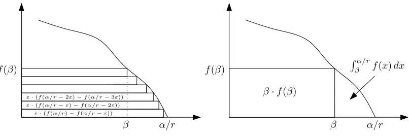
CA(Σβ) =Cf(β) = (1−f(β))·α+β·f(β) +
Z α/r
β
f(x)dx .
The first term results from the fact that in the last step of Σβ algorithmAhas to purchase
β α/r ε·(f(α/r)−f(α/r−ε))
ε·(f(α/r−ε)−f(α/r−2ε)) ε·(f(α/r−2ε)−f(α/r−3ε)) f(β)
β·f(β)
Rα/r
β f(x)dx
β α/r
[image:11.612.106.509.100.234.2]f(β)
Figure 1: The first figure illustrates the cost of algorithm A on the discrete sequence, and the second figure illustrates its cost on the continuous sequence. Since the function f is monotone, it is integrable on the compact set [β, α/r], which in turn implies that forε→0 the costs on the discrete and continuous sequence coincide.
In addition to the actual buying functionf of algorithmA, we also consider the buying functiong defined by
g(x) =r·
ln1− x α
−ln
1− 1 r
.
This buying function has the property that for allβ ∈[1, α/r]
Cg(β) = (1−g(β))·α+β·g(β) +
Z α/r
β
g(x)dx=r·β ,
as shown by the following calculation:
(1−g(β))α+β·g(β) + Z α/r
β
g(x)dx
= (1−g(β))α+β·g(β) + Z α/r
β r·
ln1−x α
−ln
1−1 r
dx
= (1−g(β))α+β·g(β) +hr·(−α+x)ln1− x α
−1iα/r
β −r·
α
r −β
ln
1− 1 r
= (1−g(β))α+β·g(β) +r·
(−α+β) ln
1− 1 r
−(−α+β) ln
1−β α
+β−α r
= (1−g(β))α+β·g(β) + (α−β)·g(β) +r·β−α r
=r·β .
Furthermore,gis a valid buying function as it is monotonically decreasing,g(α/r) = 0, and
g(1) =r·
ln
1− 1 α
−ln
1− 1 r
= 1 ,
In order to show the lower bound onA’s competitive ratio, we distinguish between two cases: eitherf(x)> g(x) for allx∈[1, α/r] or there exists anx∈[1, α/r] withf(x)≤g(x). In the former case, we set β = 1 and, according to the previous calculations, obtain that CA(Σ1) = Cf(1) > Cg(1) = r. Since the cost of an optimal offline algorithm on Σ1 is 1,
the competitive ratio of algorithm A is bounded from below by r in this case. Now let us consider the case that there exists an x∈[1, α/r] with f(x)≤g(x). In this case, we set
β = sup{x∈[1, α/r]|f(x)≤g(x)} . Since f(x)≥g(x) for all x≥β, we obtain
CA(Σβ) =Cf(β)≥Cg(β) =rβ .
Combining this with the observation that the cost of an optimal offline algorithm on the sequence Σβ isβ implies that, also in this case, the competitive ratio of Ais bounded from
below byr.
The argument above shows only that no algorithm can be strictly r′-competitive for
r′ < r(in fact, it is easy to see that no algorithm can be strictlyr′-competitive for r′< α).
However, the assumption thatA has an empty storage after each sequence Σβ allows us to
repeat an arbitrary number of sequences of this kind without affecting the argumentation above, showing that no algorithm can be better thanr-competitive. Observe that the buying function of algorithm A can be different in each repetition, which, however, cannot help to obtain a better competitive ratio because β is adopted appropriately in each repetition.
3.2. Lower Bound for Algorithms with Fixed Buying Functions
Theorem 3.2. The competitive ratio of any randomized online algorithm for the econom-ical caching problem with a fixed buying function is at least √α. This also holds for the economical caching problem without buying limits.
Proof. Let us first consider an algorithmA with an arbitrary but monotonically decreasing buying function f. We will later argue how to extend the proof to functions that are not necessarily monotonically decreasing. We construct a sequence Σ on which A is at least
√
α-competitive as follows: Σ starts with a sequence Σ′ that is similar to Σ′
1 from the proof
of Theorem 3.1 with the only exception that we decrease the efficiency from α to 1. To be precise, in every step in this sequence there is no consumption, no buying limit, and the prices are
α, α−ε, α−2ε, . . . ,1 +ε,1 ,
for a smallεwith (α−1)/ε∈N. As in the proof of Theorem 3.1, we simplify the notation by assuming that the price decreases continuously fromαto 1. The cost ofAon this sequence is
q := 1 + Z α
1
f(x)dx .
Let us assume thatf(1) = 1. Due to the construction of the sequence Σ this can only reduce the cost of A on Σ. We can also assume that f(α) = 0 because if A purchases anything at priceα, it can easily be seen that A cannot be better than α-competitive.
Now we distinguish between two cases: if q ≥ √α, then the sequence Σ is formed by appending one step with priceα, consumption 1, and no buying limit to Σ′. The cost of an
Now let us assume that q ≤ √α. After the sequence Σ′, the price increases again
from 1 to α but this time with consumption. There still is no buying limit and the prices and consumptions are as follows (the upper value indicates the price, the lower value the consumption):
1 +ε f(1)−f(1 +ε)
1 + 2ε f(1 +ε)−f(1 + 2ε)
· · ·
α−ε
f(α−2ε)−f(α−ε)
α f(α−ε)
.
Let us call this sequence Σ′′. Observe that consumptions and prices are chosen such thatA
does not purchase anything during the sequence Σ′′. The sequence Σ is formed by appending
one step with priceα, consumption 1, and no buying limit to Σ′Σ′′. On this sequence, the
optimal cost is 1+q: The optimal offline algorithm purchases an amount of 1 in the last step of Σ′ for price 1, and then it purchases in every step of Σ′′ exactly the consumption. This
way the storage is completely filled after the sequence Σ′′and no further cost is incurred in
the final step. Similar arguments as in the proof of Theorem 3.1 show that the cost during the sequence Σ′′ is q. Since algorithm A does not purchase anything during Σ′′, it has to
purchase an amount of 1 for the price of α in the final step. Hence, its total cost is q+α. Forq ≤√α, we have
q+α q+ 1 ≥
√
α+α
√
α+ 1 =
√
α .
Since f(α) = 0, algorithm A has an empty storage after this sequence. Hence, we can repeat this sequence an arbitrary number of times, proving the theorem.
If the buying functionf is not monotonically decreasing, we can, for the purpose of this proof, replace f by the monotonically decreasing functionf∗(x) := sup{f(y) |y ≥x}. An
algorithm with buying function f behaves the same as an algorithm with buying function f∗ on the sequences constructed in this lower bound with respect tof∗.
References
[1] Allan Borodin and Ran El-Yaniv.Online Computation and Competitive Analysis. Cambridge University Press, 1998.
[2] Thomas M. Cover and Erik Ordentlich. Universal portfolios with side information.IEEE Transactions on Information Theory, 42(2):348–363, 1996.
[3] Ran El-Yaniv. Competitive solutions for online financial problems.ACM Comput. Surv., 30(1):28–69, 1998.
[4] Ran El-Yaniv, Amos Fiat, Richard M. Karp, and G. Turpin. Optimal search and one-way trading online algorithms. Algorithmica, 30(1):101–139, 2001.
[5] David P. Helmbold, Robert E. Schapire, Yoram Singer, and Manfred K. Warmuth. On-line portfolio selection using multiplicative updates. InICML, pages 243–251, 1996.
[6] Erik Ordentlich and Thomas M. Cover. On-line portfolio selection. InCOLT, pages 310–313, 1996.