Master Thesis – Applied Mathematics
Average-Case Analysis of the
2-opt Heuristic for the TSP
Jaap J. A. Slootbeek
Supervisor:
Dr. B. Manthey
University of Twente
Faculty of Electrical Engineering, Mathematics and Computer Science
Abstract
The traveling salesman problem is a well-known N P-hard op-timization problem. Approximation algorithms help us to solve larger instances. One such approximation algorithm is the 2-opt heuristic, a local search algorithm. We prove upper bounds on the expected approximation ratio for the 2-opt heuristic for the traveling salesman problem for three cases. When the dis-tances are randomly and independently drawn from the uniform distribution on [0,1] we show that the expected approximation ratio is O(pnlog(n)). For instances where the distances are 1 with probability p and 2 otherwise, we prove a bound for fixed
p strictly between 0 and 1 that gives an upper bound on the number of heavy edges in the worst local optimum solution with respect to the 2-opt heuristic ofO(log(n)). For instances where the edges distances are randomly and independently drawn from the exponential distribution, we can upper bound the expected
approximation ratio byO
q
nlog3(n)
Table of Contents
1 Introduction 4
1.1 TSP and the 2-opt heuristic . . . 4
1.2 Outline of this thesis . . . 6
2 Related work 6 3 Generic on [0,1] 8 4 Discrete distribution 13 5 Exponential distribution 16 6 Simulations 22 6.1 Introduction . . . 22
6.2 TSP Model . . . 22
6.3 WLO Model . . . 24
6.4 Uniform on [0,1] . . . 26
6.5 Discrete distribution . . . 28
6.6 Exponential distribution . . . 29
7 Discussion 32
8 Conclusions 33
Bibliography 35
List of Theorems 36
A Graphical results for the discrete case 37
1
Introduction
In this section we discuss what the Traveling Salesman Problem is, how it can be solved and what approach we working on in this thesis. We also discuss the structure of this thesis
1.1
TSP and the 2-opt heuristic
Imagine you would want to take a tour to all capitals of mainland Europe. Our tour should both start and end in Amsterdam but apart from that the order is free. You find the cities in figure 1 As you are probably already thinking of some order to visit the cities in, you might be implicitly trying to minimize the distance traveled in total. After all, going from Amsterdam to Athens to Brussels to Budapest does not seem to make much sense as part of our route. This idea of minimizing the total distance covered (or for that matter, total cost) leads us to the Traveling Salesman Problem (TSP). The problem is defined as follows:
Definition 1.1 (Traveling Salesman Problem (TSP)) An instance of TSP is a complete graph with distances for all edges. A solution is a Hamilton cycle. That is, a solution is a cycle visiting all nodes exactly once. The goal is to minimize the sum of the edge distances on such a cycle.
[image:4.595.224.395.472.614.2]In the remainder of this thesis we denote the number of nodes in an instance byn. From this we get some requirements. Firstly, the route has to be circular, that is, it has to end where it started. Secondly, it has to visit each city exactly once. Most importantly however, there has to be no other route that meets these requirements but that is shorter.
Figure 1: European capitals that should be included in the tour
A naive method for finding a solution is merely trying every possible route. If we want to visit ncities and we know where we want to start there are about (n−1)!/2 different routes possible. While this may work for small instances, for larger instances this leads to issues such as extremely long processing times. For instance, for the 40 cities in figure 1 there are over 1046possible routes,
To look at the complexity of the problem, we must consider the decision version of the TSP. Instead of asking for the cheapest route we ask to find a route that is cheaper than a valuekif it exists. For completeness we define the problem as follows.
Definition 1.2 (Traveling Salesman Problem decision version (TSP-d)) An instance of TSP-d is a complete graph with distances for all edges. Also given is a value K. A solution is a Hamilton cycle. The goal is whether to decide if there exists a solution where the sum of the edge distances on such a cycle is at mostK.
In 1972 Karp showed that the TSP-d is N P-complete and TSP N P-hard. This means that, assuming P 6= N P we see that TSP cannot be solved in polynomial time. It appears that we need to limit our expectations for the algorithms we can find. Nevertheless, the question whether
P =N P or not is still an open question.
Over time several methods that solve the TSP have been developed. The brute force method we saw before runs has a running time in O(n!), since the work on a given route is done in polynomial time. Apart from the brute force method one of the options is dynamic programming. An algorithm by Held and Karp (1962) uses dynamic programming to solve the TSP. It also uses the property that every subpath of a path of minimum distance is itself also of minimum distance. The running time for this algorithm is inO(n22n)). Other options include the successful
branch-and-cut approach, as used in Concorde (Applegate et al., 2011). Using the branch-and-cut approach with multiple separation routines and column generation Concorde is able to solve large instances of the TSP. Concorde was able to solve an instance with 85900 nodes to optimality (Applegate et al., 2009).
The previous algorithms all find the optimal solution. In some cases we accept a near-optimal solution instead of a fully optimal solution if the near-optimal solution is found in less time. In this case we use heuristics. These aim to find good (enough) solutions within reasonable time. We categorize these heuristics into two main categories, constructive heuristics and iterative improvement heuristics. Constructive heuristics aim to build a tour from scratch. An example of such a heuristic is the nearest neighbour heuristic (Kizilate¸s and Nuriyeva, 2013). At every point the salesman selects the closest other node that has not yet been visited until a full tour is found. The algorithm we analyze in this paper falls into the iterative improvement category.
One of the more common ways to achieve iterative improvement by using local search (Aarts and Lenstra, 2003). In local search, each solution has a neighbourhood and in each iteration we select the best solution in the neighbourhood of the current solution. More formally, each optimization problem instance is a pair (S, f) whereS contains all solutions andf :S→Rgives each solution a value. If we consider a minimization problem, like the TSP, we want to find the solutions?∈S
with the lowestf(s?). Let N(s) be the neighbourhood of s. In each step of the local search we
look for the best solution in the neighbourhood of the current solution. More formally, ifscis our
current solution we want to find ˜ssuch that for alls0 in N(sc) we have f(˜s)≤f(s0). If the best
solution we find is the current solution then we have found a local optimum. This locally optimal solution does not have to be the global optimal solution, that is, the best solution overall. Local search is a broad technique that has been applied to several fields. We tailor it to our specific problem by defining the neighbourhoods. If needed we can also define how the initial solution is created.
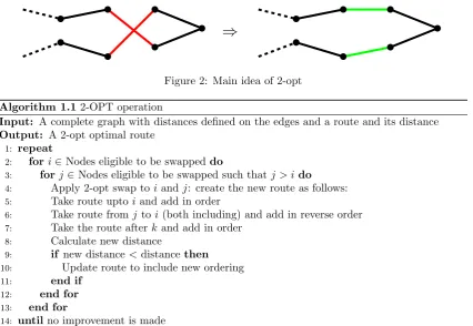
neighbourhood of a solutionsis all solutions where two edges have been removed and replaced by two other edges to create a feasible Hamilton cycle. This idea was introduced by Croes (1958). The algorithm is shown as Algorithm 1.1. Note that this algorithm only finds local optima under the 2-opt neighbourhood. This means that we cannot perform another 2-opt step on the route to find a better route. However, this does not guarantee an optimal solution for the TSP.
[image:6.595.91.518.175.469.2]⇒
Figure 2: Main idea of 2-opt
Algorithm 1.12-OPT operation
Input: A complete graph with distances defined on the edges and a route and its distance Output: A 2-opt optimal route
1: repeat
2: fori∈Nodes eligible to be swappeddo
3: forj∈Nodes eligible to be swapped such thatj > ido
4: Apply 2-opt swap toi andj: create the new route as follows:
5: Take route uptoiand add in order
6: Take route fromj toi(both including) and add in reverse order
7: Take the route afterk and add in order
8: Calculate new distance
9: if new distance<distance then
10: Update route to include new ordering
11: end if
12: end for 13: end for
14: untilno improvement is made
1.2
Outline of this thesis
The remainder of this thesis is in broad terms divided into two parts. In the first part (Sections 3 upto 5) we present the theoretical results. We analyse three different classes of instances, firstly, instances where the edge distances are drawn from a slightly generalized version of the uniform distribution on [0,1] in Section 3. Secondly, we consider in Section 4 instances where the edges have a distance of either 1 or 2, this means we consider a discrete distribution. As third case we consider instances where the edge distances are drawn from the exponential distribution in Section 5. The second part contains the simulation results. In Section 6 we compare the theoretical results to experimental observations. After that we will discuss our results and findings in Section 7 and present our conclusions in Section 8.
2
Related work
field. We discuss several results related to the average-case approximation results we present as well as to other approximation results.
This thesis expands on a paper by Engels and Manthey (2009). They proved that for instances with nnodes and edge weights drawn uniformly from [0,1] and independently the expected ap-proximation ratio isO(√n·(log(n)3/2). For this case we prove a better upper bound in the next section.
Chandra et al. (1999) have proved that the worst-case performance ratio for TSP instances where the triangle inequality holds is at most 4√nfor allnand at least 14√nfor infinitely manyn. On the other hand Grover (1992) proved that for any symmetric TSP instance any 2-optimal route has a length that is at most as high as the average length of all tours.
We can prove results in the forms of worst-case approximation ratios, which can be too pessim-istic due to the very very specific features in the instances and the average-case approximation ratios, which can be dominated by completely random instances that do not represent the real-life instances well. Smoothed analysis Spielman and Teng (2004) forms a hybrid of both these cases. We let an adversary specify an instance. Instead of using that instance directly (which is the case in the worst-case analysis) we apply a slight (random) perturbation to it. If we take the expected value of this random perturbation we get from the smoothed performance the expected perform-ance. The idea behind this approach is that in practice instances are usually subject to a small amount of noise. When we look at the title of the paper by Spielman and Teng (2004), ”Smoothed Analysis of Algorithms: Why the Simplex Algorithm Usually Takes Polynomial Time” we get one of the results in this paper. It can be very confusing to observe a good performance but having a quite bad theoretical bound. As the theoretical bound is often due to some unlikely or unrealistic instances, using this methods should allow for more realistic conclusions. This method has also been employed for the 2-opt heuristic.
An important measure when using the opt heuristic is how many steps are needed to reach a 2-opt 2-optimal solution. Englert et al. (2014) showed that expected length of any 2-2-opt improvement path is ˜O(n4+1/3·φ8/3). For intuition you can think of φ to be proportional to 1/σd, being
a perturbation parameter. In other cases, such as when the initial tour is constructed by an insertion heuristic, this upper bound can be improved further. Manthey and Veenstra (2013) look at the Euclidean TSP which means that cities are placed on [0,1]d. The distances then depend on the locations of the points: we can for example use the Euclidean or the Manhattan norms to determine the distances. The instances are perturbed by independent Gaussian distributions with mean 0 and standard deviationσ. Ford-dimensional instances ofnpoints the bound on the number of steps needed is O(√dn4D4
maxσ−4) for the Euclidean norm and O(d2n4Dmaxσ−1) for
the Manhattan norm. In thisDmax such thatx∈[−Dmax;Dmax]d with a probability of at least
1−1/n! for all pointsx.
Englert et al. (2014) also showed an upper bound on the expected approximation ratio of the Euclidean TSP with respect to all Lp metrics of O(d
√
φ). K¨unnemann and Manthey (2015) also worked on the approximation ratio. They were able to prove that for instances ofnpoints in [0,1]d
perturbed by Gaussians of standard deviationσ≤1 the approximation ratio is inO(log(1/σ)).
3
Generic on [0
,
1]
The goal of this section is to find a result for instances where the distances are drawn from a standard uniform distribution. However, as the extension of this proof to a more general case was found to give the same result, we present this generalisation. We find a result gives a bound on the growth ofE(WLOn/OPTn) where WLOn is the worst local optimum that can be attained by
the 2-opt operation and OPTn is the optimal TSP solution
Assume we have a generic distributionG which can take only values on [0,1] with a probability density functionf(x) and a cumulative distribution functionF(x) defined. We have the following properties:
• F(0) = 0, by definition
• F(1) = 1, by definition
• F(x) is non-decreasing, by definition
• F(x)≥x
• f(x) is non-increasing
Examples of this includeF(x) =x(uniform on [0,1]) andF(x) =√x. Before we can start looking at the specifics for this set of instances we first need to look at how we are going to count edges.
Lemma 3.1 There exist at least mn64 pairs of edges where at least one edge is heavy and where the edges that are inserted by performing a 2-opt operation on these edges are disjoint.
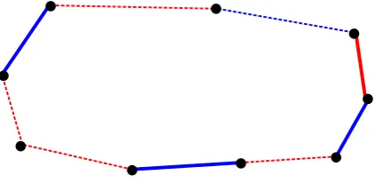
[image:8.595.195.411.596.699.2]Proof. We call an edge heavy if it has a weight greater thanη. We want to find a lower bound on the amount of pairs of edges where at least one edge is heavy and where the edges that will be inserted by performing the 2-opt operation (on those edges) are disjoint. If a combination of two edges have the latter property we call that combinationindependent. We want to colour the edges such that any pair of edges with colour blue forms to an independent combination. We colour the edgesred andbluesuch that there are no two adjacent blue edges. For an odd number of edges this leads to two adjacent red edges. This colouring has the property that when we use the blue edges the edges that will be inserted by performing the 2-opt operation (on those edges) are disjoint. Note that this colouring can be rotated over the edges in the cycle without losing its properties. However we choose the colouring that has the most heavy blue edges.
Figure 3: A possible colouring, continuous lines are heavy, dashed lines are not heavy.
0.5·(m−1) heavy edges that are blue. We use the rough boundmn/64 for the total amount of possible independent combinations of a heavy edge and any other edge, taking into account that there some combinations could be counted double.
Consider a combination with blue edges eand e0 with eheavy which is possible without loss of generality. When performing the 2-opt operation these edges are replaced by the edgesf andf0 as determined by the 2-opt operation. We know that ifw(e) +w(e0)> w(f) +w(f0) thatH is not
a locally optimal tour. Since the weights are non-negative we know thatw(e) +w(e0)≥η. So, if w(f) +w(f0)< ηwe know thatH is not optimal. We use this frequently in the remainder of this thesis.
We now have a lower bound on how many pairs we can find with properties we find desirable. Using this we are able to bound the probability that a cycle with some heavy edges is locally optimal under the 2-opt operation.
Lemma 3.2 Let H be any fixed Hamiltonian cycle and letη∈(0,1]. Assume H contains at least
m ≥4 edges of weight at least η. The weights of the edges are random variables taken from G. Let the weights of the edges on the cycle be known. Then
P(H is locally optimal)≤e− F2 (η)mn
64
Proof. Consider a pair of edges from lemma 3.1. This is a independent pair of edges eand e0 with eheavy which is possible without loss of generality. When performing the 2-opt operation these edges are replaced by the edgesf andf0 as determined by the 2-opt operation. We know that ifw(e) +w(e0)> w(f) +w(f0) that H is not a locally optimal tour. Since the weights are non-negative we know that w(e) +w(e0) ≥ η. So, if w(f) +w(f0) < η we know that H is not optimal.
Now we determineP(w(f) +w(f0)< η) forη∈[0,1]:
P(w(f) +w(f0)< η) =
Z η
0
P(w(f) +w(f0)< η|w(f) =x)dx
=
Z η
0
P(w(f0)< η−x|w(f) =x)dx
=
Z η
0
F(η−x)f(x)dx
≤
Z η
0
F(η)f(x)dx
=F(η)·
Z η
0
f(x)dx
=F(η)·(F(η)−F(0))
=F2(η)
where the inequality follows from the cumulative distribution function being non-decreasing.
So for a combination an improving 2-opt operations is possible with probabilityF2(η). In order for a tourH to be optimal, it cannot have any improving 2-opt operations, in particular not for themn/64 independent combinations we found. That means that
P(H is locally optimal)≤ 1−F2(η) mn
64 ≤e−F2 (64η)mn (1)
Now we know how the probability of a tour being optimal can be estimated. Now we can look into the probability of the worst solution generated by 2-opt being over a certain weight. For this we use the following lemma.
Lemma 3.3 For any c >8 and a distributionGas above, we have
P
WLOn≥6c
p
nlog(n)≤exp
nlog(n)
1− 1
64c
2
Proof. Definemi = 3−in, ηi = 2iη and η =c· p
log(n)n−1. We are going to look at a tour H
which contains at mostmi edges of weight at least ηi. First, if i≥log(n) we have mi <4 and
ηi >1. Because the weights are at most 1 it is sufficient to consideri ∈[0, . . . ,log(n)−1]. If a
tourH contains at mostmi edges of weight at leastηithen
w(H)≤
log(n)−1 X
i=0
miηi+1.
We can see this as follows: for eachiwe count the number of edges with weight more thatηi, we
count these with weightηi+1. For some edges this may be too low but these will be counted again
for a higheri. Hence we achieve an upper bound on the weight of the tour.
We have
miηi+1= 2
2
3
i
ηn= 2c
2
3
i
p
nlog(n).
Using this, we have
w(H)≤
log(n)−1 X
i=0
miηi+1=
log(n)−1 X i=0 2c 2 3 i p
nlog(n) = 2cpnlog(n)
log(n)−1 X
i=0
2
3
i
≤6cpnlog(n)
where the last inequality uses the geometric series
We now want to estimate the probability that the tour H which contains at most mi edges of
weight at leastηi. For the probability of this to happen, we refer back to Lemma 3.2 and first look
at the case for a fixedi. Fix any tourH. The probability thatH is locally optimal provided it contains at leastmiedges of weight at leastηi(call these conditions?i) is at most exp(−F
2(ηi)m
in
64 ).
Thus,
P(H is optimal under?i)≤exp
−F
2(η
i)min
64
= exp
−−F
2(2iη)3−in2
64
We use Boole’s inequality to bound the probability thatH is locally optimal from above, provided there exists ani∈[0, . . . ,log(n)−1] for whichH contains at leastmi edges of weight at leastηi.
Again using Boole’s inequality, we determine an upper bound to the probability that one of then! possible tours is locally optimal, provided that it contains at leastmi edges of weightηi for some
i. This probability is at most
n!·log(n)·exp
−−F
2(2log(n)η)3−log(n)n2
64
We work on this expression to find
P
WLOn≥6c p
nlog(n)≤n!·log(n)·exp
−F
2(2log(n)η)3−log(n)n2
64
≤nn·exp
−F
2(2log(n)η)n2
64·3log(n)
= exp
nlog(n)−F
2(2log(n)η)n2
64·3log(n)
= exp
n
log(n)−F
2(2log(n)η)n
64·3log(n)
For this probability to go to 0 for largen, we need 64·3log(n)·log(n)≤F2(2log(n)η)n. This is true
if 64·3log(n)·log(n)
n ≤F
2(2log(n)η) or
8·√3
log(n)rlog(n)
n ≤F(2
log(n)η) =F c
·2log(n)· r
log(n) n
!
We can see this is at least true if F(x)≥xforx∈(0,1] andc >8. In this case, we can use the following bound:
F2(2log(n)η)n 64·3log(n) ≥
4log(n)·η2n 64·3log(n) =
1 64
4 3
log(n)
c2log(n) n n≥
1 64c
2log(n)
The result follows: For anyc >2 and a distributionGwithF(x)> xforx∈(0,1] we have
P
WLOn ≥6c p
nlog(n)≤exp
nlog(n)
1− 1
64c
2
. (2)
We also note here that for c >8 this probability is strictly decreasing in n and approaches zero at least exponentially fast asnincreases.
We remark that, with our constraint onF(x) andc, the probability that the worst local optimum worse than 6cpnlog(n) goes to zero quickly for highn. We also present the following lemma to bound the optimal solution of an instance.
Lemma 3.4 For any n≥2 andc∈[0,1], we have P(OPTn≤c)≤nF(c)cn−1f(0)n−1
Proof. First we look atP(w(H)≤c). We claim that for a instance withnnodes we have
P(w(H)n≤c) =
F(c)cn−1f(0)n−1
(n−1)! (3)
We prove this using induction. Forn= 1 we get
Now for the induction step. Assume (3) is true forn≤k−1. Now we work onP(w(H)k≤c).
P(w(H)k ≤c) =
Z c
x=0
P(w(H)k−1≤c−x)f(c)dx
≤
Z c
x=0
P(w(H)k−1≤c−x)f(0)dx
=f(0)
Z c
x=0
P(w(H)k−1≤c−x)dx
IH
=f(0)
Z c
x=0
F(c−x)(c−x)k−2f(0)k−2
(k−2)! dx
≤f(0)k−1
Z c
x=0
F(x)(x)k−2 (k−2)! dx
≤f(0)k−1F(c)
Z c
x=0
(x)k−2
(k−2)!dx
=f(0)
k−1F(c)ck−1
(k−1)!
Now we use Boole’s inequality to bound the probability that there exists a tour withw(H)≤cto find the result.
Theorem 3.5 (Result for general distribution) Fix a distribution G for the weights of the edges withFG(x)≥xfor0< x≤1. We have
E
WLO
n
OPTn
∈Opnlog(n)
Proof. Assume WLOn/OPTn > 6c2 p
nlog(n) for c > 8. Then WLOn ≥ 6c p
nlog(n) or OPTn≤ 1c. The probability that WLOn≥6c
p
nlog(n) is given by Lemma 3.3. The probability that OPTn < 1c is less than F(1/c)f(0)n−1(1/c)1−nn. The probability of either of these events
happening is at mostF(1/c)f(0)n−1 1
c
n−1
n+ exp nlog(n) 1− 1 64c
2
forc >8. Then we know for allξsuch thatξ > f(0)4 andξ >642 that
WLOn
OPTn
≤6pnlog(n)·
Z ∞
ξ
cP(c)dc2+O(pnlog(n)) (4)
We perform the substitutionx=c2 and find
WLOn
OPTn
≤3pnlog(n)·
Z ∞
√ ξ
P(√x)dx+O(pnlog(n)) (5)
We calculateR∞ x=√ξP(
√
x)dxby splitting it into the two separate parts
Z ∞
x=√ξ
P(√x)dx=
Z ∞
x=√ξ
F(1/√x)f(0)n−1
1
√
x
n−1
ndx+
Z ∞
x=√ξ
exp
nlog(n)
1− 1
64x
We work on these independently to find
Z ∞
x=√ξ
F(1/√x)f(0)n−1
1
√
x
n−1
ndx=
2nF√1 x
ξ34−n4f(0)n−1
n−3 and
Z ∞
x=√ξ
exp
nlog(n)
1− 1
64x
dx= 64n
−n√ξ
64 +n−1
log(n)
Combining these we find
Z ∞
x=√ξ
P(√x)dx=
2nF√1 x
ξ34−n4f(0)n−1
n−3 +
64n−n
√ ξ
64 +n−1
log(n)
=F(1/
√
ξ)ξ34
f(0) ·
f(0)
ξ14
n
· 2n
n−3 + 64n−n
√ ξ
64 +n−1
log(n) .
This function goes to zero exponentially fast asnincreases provided we indeed have thatξ >642 and ξ > f(0)4 . We can say that Rc∞=ξcP(c)dc2 ∈ O(1). This combined with (4) leads to the following result E WLO n OPTn
≤Opnlog(n)·O(1) +O(pnlog(n))∈Opnlog(n) (6)
Corollary 3.6 (Uniform distributions) Let the weight of the edges be drawn from the any uniform distribution on[0, χ] with0< χ≤1. We have
E
WLO
n
OPTn
∈Opnlog(n)
Corollary 3.7 (Standard uniform distribution) Let the weight of the edges be drawn from the standard uniformdistribution, on[0,1]. We have
E
WLO
n
OPTn
∈Opnlog(n)
4
Discrete distribution
In this section we will consider graphs where the distances between points are one of two values. This is a discrete distribution. We find a result that bounds to growth of the number of heavy edges used in the Worst Local Optimum solution under the 2-opt operation. As there are only two choices for the heights, a heavy edge is an edge whose weight is the higher of the two. In this section we use the weights 1 and 2. Edges with weight 2 are therefor calledheavy.
Consider a complete graph with n vertices where the weights of the edges are independently determined as follows:
w(e) =
(
Lemma 4.1 Let H be any fixed Hamiltonian cycle. Assume H contains at least m edges of weight 2. Let the weight for the edges onH be known. The weights for the other edges are iid with
w(e) = 1w.p. pandw(e) = 2w.p. 1−p. Then
P(H is locally optimal)≤(1−ξ(p)) nm
64 ≤e−
ξ(p)nm
64
withξ(p) = 2p−3p2+ 2p3
Proof. By Lemma 3.1 there are at leastmn/64 independent pairs with at least one heavy edge. Look at such a combination (e, e0) withw(e) = 2. 2-opt will be able to improve the tour to include the edges (f, f0) instead of (e, e0) ifw(e) +w(e0)> w(f) +w(f0). Looking closer at this we see:
w(e) +w(e0)> w(f) +w(f0)⇒2 +w(e0)> w(f) +w(f0)⇒w(f) +w(f0)−w(e0)<2
Since we know the probabilities for the weights of the edge we can fill out the following table:
w(f) w(f0) w(e) w(f) +w(f0)−w(e) w(f) +w(f0)−w(e0)<2 Probability
1 1 1 1 X p3
1 1 2 0 X p2(1−p)
1 2 1 2 ×
1 2 2 1 X p(1−p)2
2 1 1 2 ×
2 1 2 1 X p(1−p)2
2 2 1 3 ×
2 2 2 2 ×
Total: p3+p2(1−p) + 2p(1−p)2
p3+p2(1−p) + 2p(1−p)2=p 2p2−3p+ 2
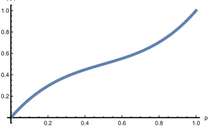
This means that the probability that a tourH withmedges of weight two is is locally optimal is bounded from above by 1−2p+ 3p2−2p3nm64. Denote 2p−3p2+ 2p3 (see figure 4) as ξ(p) to
simplify notation. We then get
0.2 0.4 0.6 0.8 1.0 p
0.2 0.4 0.6 0.8 1.0
[image:14.595.193.405.544.683.2]ξ(p)
Figure 4: A plot of ξ(p) for 0≤p≤1
P(H is locally optimal)≤(1−ξ(p)) nm
64 ≤e−
ξ(p)nm
64 (7)
Lemma 4.2 For any mwe have
P(W LOn≥n+m)≤exp
n
log(n)−1
4mξ(p)
Proof. We are going to look at a tour H which contains at mostm edges of weight 2. We can bound the weight of such a tour from above as
w(H)≤X e∈E
w(e) =n+m.
We refer back to Lemma 4.1 to find the probability of a tour of this weight being locally optimal. The probability that H is locally optimal, given that it contains at least m edges of weight 2 (denote this condition by♦) is at most exp(−1
64ξ(p)nm).
We use Boole’s inequality to bound the probability that one of the n! possible tours is locally optimal from above, provided that it contains at leastmedges of weight 2. We get
P(H is locally optimal under♦)≤n!·exp
−1
64ξ(p)nm
.
By boundingn! from above bynn= exp(nlog(n)) we find the result
P(W LOn≥n+m)≤exp
n
log(n)− 1
64mξ(p)
We note that this probability goes to 0 for largenif log(n)≤ 1
64mξ(p), from which we gather that
that is the case if the number of heavy edges is larger than log(n).
Theorem 4.3 (Result for the discrete case) Denote by#Heavythe number of edges of weight 2 in the Worst Local optimum. For a constant p we have
E(#Heavy)∈O(log(n)).
Proof. Assume we have more than c·log(n) heavy edges with c ≥ 5 and c ≥ 5
ξ(p). Since
clog(n)>log(n) we can use Lemma 4.2. Thus we find that the probabilityPc of this happening
is at most
expnlog(n)1−c
4ξ(p)
.
In the case we have more thanclog(n) heavy edges, we will still no more thannheavy edges. It follows that
E(#Heavy)≤n·Pc+O(log(n)).
We know thatPc≥exp(nlog(n)(1−5/4) = exp(−0.25nlog(n)) =n−n/4because of the constraints
5
Exponential distribution
After looking at the uniform distribution and discrete cases we also look at instances where the distances are drawn from the exponential distribution. In this section we will first see how we are going around the issue that the distances do not have an upper bound. After that we look for a order bound onE(WLOn/OPTn).
Consider a complete graph withnvertices where the weights of the edges are independently drawn from the exponential distribution with parameterλ= 1. We also assume we have at least 4 edges in the Hamiltonian cycles, son≥4.
Remember that random variables with an exponential distribution can reach arbitrarily large values. We want to have a bound for this such that the probability of an edge having a weight over the bound is very small. First we find a bound on the probability that the maximum edge weight is more thanq.
Lemma 5.1
P
max
e∈Ew(e)> q
≤2ne−q forq >0.25
Proof. We use that the weights of the edges are independent.
P(max
e∈Ew(e)> q) = 1−P(maxe∈Ew(e)≤q)
= 1−P(w(e1)< q, w(e2)< q, . . . , w(en)< q)
= 1−P(w(e1)< q)P(w(e2)< q). . .P(w(en)< q)
= 1−(1−e−q)n
= 1−(1 + (−e−q))n
≤1−e−2e−q
n
by using 1 + 0.5x≥exfor −1.5≤x≤0
= 1−e−2ne−q
≤1− 1−2ne−q
by usingex≥1 +xfor allx
= 2ne−q
We bound the weight atκ= 100 log(n) and findP(maxe∈Ew(e)> κ)≤2n−99 using Lemma 5.1.
We refer back to this bound on the weight of edges as theκ-bound.
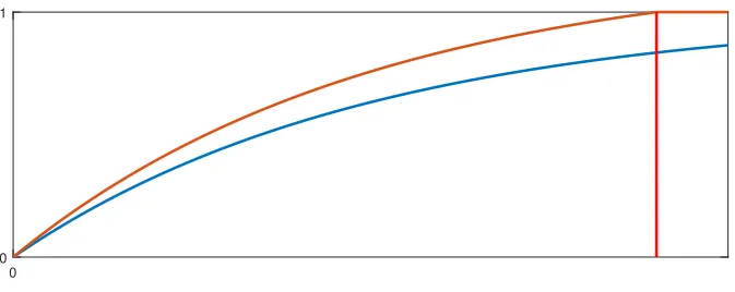
In this case we have to work with a slightly different cumulative density function for the weights of the edges. The mass that in the exponential distribution on values overκis now equally divided over the remainder. This means that the cumulative density function is a scaling of the original one. See Figure 5 for a graphical representation. We haveP(w(e) = q)L =c·P(w(e) = q) and
P(w(e)≤q)L=c·P(w(e)≤q) where the subscriptLindicates the limited version and c is very
close to 1. However, to make notation cleaner we usec= 2.
0 0 1
Figure 5: We choose the red vertical line as our κ-bound. The cumulative density function is scaled with a constant factor being 1
F(κ) so it reaches one exactly atκ.
Lemma 5.2 Let η > 0. Let H be any fixed Hamiltonian cycle. Assume H contains at least m
edges of weight at least η. The weights for the other edges are iidExp(λ).
P(H is locally optimal)≤4(η+ 1)e−η mn
4
Proof.
We call an edge heavy if it has a weight greater thanη. By Lemma 3.1 there are at leastmn/64 independent pairs of edges where at least one edge is heavy. Consider such a pair eand e0 with eheavy which is possible without loss of generality. When performing the 2-opt operation these edges are replaced by the edgesf andf0 as determined by the 2-opt operation. We know that if w(e)+w(e0)> w(f)+w(f0) thatH is not a locally optimal tour. Since the weights are non-negative we know thatw(e) +w(e0)≥η. So, if w(f) +w(f0)< η we know that H is not optimal.
Now we determineP(w(f) +w(f0)< η|κ-bound), the probability that the edges that are inserted
by a 2-opt operation have a low enough weight.
P(w(f) +w(f0)≤η |κ-bound)≤
Z η
0
2·F(x)·2·f(η−x)dx
=
Z η
0
4 1−e−x
e−(η−x)
= 4
Z η
0
e−η+xdx−
Z η
0
e−ηdx
= 4
Z η
0
e−η+xdx−ηe−η
= 4
Z η
0
e−xdx−ηe−η
= 4 −e−xη0−ηe−η
= 4−4(η+ 1)e−η.
For an independent combination of edges where one is heavy an improving 2-opt operations is possible with probability at most 1−(η+ 1)e−η. In order for a tourH to be optimal, it cannot
we found. This means that
P(H is locally optimal)≤4(η+ 1)e−η mn
64 −3≤4(η+ 1)e−η
mn
64 (8)
Lemma 5.3 For any c≥50 we have
P
WLOn≥20c
p
nlog(n)·log(n)≤cn10exp
nlog(n)−c q
log(n)
n n
2
64
Proof. We find the probability that a cycleH is over a certain weight. For that we need to use a way to calculate the weight of a constructed cycle for which we use Lemma 5.2. Let the classesi run from 0 upwards. We are going to look at a tourH which contains at mostmi edges of weight
at leastηi. For each iwe count the number of edges with weight more that ηi. We count these
with weightηi+1. For some edges this may be too low but these are counted again for a higheri.
This gives the following expression for the weight
w(H)≤ ∞ X
i=0
miηi+1.
Definemi= 2−in, ηi= 2iη andη =c· p
log(n)n−1. Because the weights are at most 100 log(n)
under theκ-bound it is sufficient to consideri ∈[0, . . . ,10 log(n)−1], as when i≥10 log(n) we haveni > κ. If a tourH contains at mostmi edges of weight at leastηi then
w(H)≤
10 log(n)−1 X
i=0
miηi+1.
We have
miηi+1= 2ηn= 2c p
nlog(n).
As we use theκ-bound we find
w(H)≤
10 log(n)−1 X
i=0
miηi+1=
10 log(n)−1 X
i=0
2cpnlog(n) =cpnlog(n)
10 log(n)−1 X
i=0
2≤20cpnlog(n)·log(n).
We now want to estimate the probability that the tour H which contains at most mi edges of
weight at leastηi is optimal. For the probability of this to happen, we refer back to Lemma 5.2.
The bound we get is 4(η+ 1)e−ηmn
10.
We first look at the case for a fixedi. Fix any tour H. The probability that H is locally optimal provided it contains at least mi edges of weight at least ηi (call these conditions?i) is at most
4·(ηi+ 1) exp −ηim10in
. Thus,
P(H is optimal under ?i)≤4·(ηi+ 1) exp
−ηi
min
64
= 4·(2iη+ 1) exp
−ηn
2
64 ·
We use Boole’s inequality to bound the probability thatH is locally optimal from above, provided there exists an i∈[0, . . . ,10 log(n)−1] for whichH contains at leastmi edges of weight at least
ηi. Again using Boole’s inequality, we determine an upper bound to the probability that one of
then! possible tours is locally optimal, provided that it contains at leastmi edges of weightηi for
somei. This probability is at most
4·n!·10 log(n)·(210 log(n)η+ 1) exp
−ηn 2 64 · .
We work on this expression to find
P
WLOn≥20c p
nlog(n)·log(n)|κ-bound≤4·n!·10 log(n)·(210 log(n)η+ 1) exp
−ηn
2
64
≤nn·10 log(n)·(210 log(n)η+ 1) exp
−ηn
2
64
= (210 log(n)η+ 1) exp
nlog(n)−ηn
2
64
= 210 log(n)c
r
log(n) n + 1
!
exp
nlog(n)−c q
log(n)
n n
2
64
We note that forn → ∞ P
WLOn≥20c p
nlog(n)|κ-boundgoes to zero. When c ≥50 the maximum is beforen= 5.
We include the properties of theκ-bound to find
P
WLOn≥20c q
nlog3(n)
=P
WLOn≥20c q
nlog3(n)|κ-bound
+P
WLOn ≥20c q
nlog3(n)|noκ-bound
≤ 210 log(n)c
r
log(n) n + 1
!
exp
nlog(n)−c q
log(n)
n n 2 64 · 1− 1 2n99
+ 1·
1
2n99
where the last 1 is an upper bound for any probability.
Whenngrows larger the left side of the above equation dominates. From this we conclude
P
WLOn≥20c p
nlog(n)·log(n)≤ 210 log(n)c
r
log(n) n + 1
!
exp
nlog(n)−c q
log(n)
n n
2
64
≤e10 log(n)cexp
nlog(n)−c q
log(n)
n n
2
64
≤cn10exp
nlog(n)−c q
log(n)
n n
2
64
As we have a result on WLOn and we want to work on E(WLOn/OPTn) we also need to find a
Lemma 5.4
P(OPTn ≤c)≤cn
Proof. We are going to determine the probability that a cycle is lighter than c. With that, we can determine the probability that all of then! cycles are lighter thanc. The result we find also holds for the shortest cycle.
We have for a cycleC
P(w(e1) +w(e2) +. . .+w(en)≤c)≤
cn n! We prove this by induction. For the base case we have
P(w(e1)≤c) =
Z c
0
e−xdx
≤
Z c
0
1dx
= c
1
1! =c
Now we assume thatP(w(e1) +w(e2) +. . .+w(en−1)≤c)≤cn−1/(n−1)!. If this is the case we
have
P(w(e1) +w(e2) +. . .+w(en)≤c) =
Z c
0
e−xP(w(e1) +w(e2) +. . .+w(en−1)≤c−x) dx
≤
Z c
0
e−x(c−x)
n−1
(n−1)! dx
≤
Z c
0
(c−x)n−1
(n−1)! dx
=
Z c
0
xn−1 (n−1)! dx
=
xn
n!
c
0
= c
n
n!
We use the union bound to find
P(weight of some cycle≤c)≤n!·
cn
n! =c
n
Now we prove the final result of this part.
Theorem 5.5 (Result for the exponential case) We have
E
WLO
n
OPTn
∈O
q
nlog3(n)
Proof. Assume WLOn/OPTn >20c2 q
nlog3(n) for c >200. Then WLOn ≥20c q
nlog3(n) or
OPTn≤1c. The probability that WLOn ≥20c q
nlog3(n) is given by Lemma 5.3. The probability
that OPTn <1c is at mostc−nby Lemma 5.4. The probability of either of these events happening
is at most
P(c) =cn10exp
nlog(n)−c q
log(n)
n n
2
64
+c−
n
We then have two cases, WLOn/OPTn >20c2 q
nlog3(n) and WLOn/OPTn ≤20c2 q
nlog3(n). We have a probability limiting the first case and for the second case we have a bound on the value of the ratio. We will see that the probability for this first case goes to zero very fast.
This leads to
WLOn
OPTn ≤20
q
nlog3(n)·
Z ∞
4000
cP(c)dc2+O
q
nlog3(n)
(9)
and after substitutingx=c2we find
WLOn
OPTn ≤10
q
nlog3(n)·
Z ∞
4000
P(√x)dx+O
q
nlog3(n)
. (10)
We calculateR∞ x=4000P(
√
x)dx by splitting it into the two separate parts
Z ∞
x=4000
P(√x)dx=
Z ∞
x=4000
√
x−ndx+
Z ∞
x=4000
√
xn10exp
nlog(n)− √
x
q log(n)
n n
2
64
dx.
We work on these independently to find
Z ∞
x=4000
√
x−ndx= 2
6−5n
2 53− 3n
2
n−2 and
Z ∞
x=4000
√
xn10exp
nlog(n)− √
x
q log(n)
n n 2 64 dx =
4096nn+4e18(−5)
√
5 2n
2qlog(n)
n
125n3log(n) + 80√10n2qlog(n)
n + 256
log(n)
n
3/2
Combining these we find
Z ∞
x=4000
P(√x)dx= 2
6−5n
2 53− 3n
2
n−2 +
4096nn+4e18(−5)
√
5 2n
2qlog(n)
n
125n3log(n) + 80√10n2qlog(n)
n + 256
log(n)
n
The dominating term is exp
1 8(−5)
q 5 2n
2qlog(n)
n
which for n > 4 is always smaller than
exp(−n). Thus this function goes to zero at least exponentially fast as n increases for n > 4. We can say thatR∞
c=200P(c)dc∈O(1). This combined with (10) leads to the following result
E
WLO
n
OPTn
≤O
q
nlog3(n)
·O(1) +O(
q
nlog3(n))∈O
q
nlog3(n)
(11)
6
Simulations
6.1
Introduction
After finding theoretical results we also want to verify our results experimentally. For this we ran some simulations. In these simulations we use integer linear programs to solve different instances both to optimality as well as to the worst local optimum with respect to the 2-opt neighbourhood. First we describe the models and procedures. The project files are based on the material by Bodo Manthey for the course “Optimization Modeling”. We use the software AIMMS to model the problems and CPLEX 12.6.2 to solve them. The experiments were run on a Windows 10 desktop machine with an Intel core i5 3.2 GHz processor and 16 GB of RAM. The time results may not be entirely consistent because of the usage of a desktop on which other applications are running (e.g. windows update). While the goal of the experiment is not to compare times, it may have affected the size of the instances that can be solved. However, as we see later the problems itself are very large and we expect this effect to be negligible.
We recall that solving the TSP is already an NP-hard problem. When solving for the worst local optimum we need another problem. We want to find a solution to the TSP (that is, a tour that visits each node exactly once). However, this solution also needs to be 2-optimal. That means there cannot be an improving 2-opt operation. We formalize this notion as follows:
If (u, v) and (x, y) are containted in the tour, thendu,v+dx,y ≤du,x+dy,v. (12)
where u, v, x, y are distinct nodes, Tour(u, v) is true if and only if the edge (u, v) is used and
Distance(u, v) gives the distance from uto v. We clearly see the 2-opt idea in this condition. To solve for the worst local optimum (WLO) we have instances like in the TSP. Solutions are tours that visit all nodes exactly once and meet condition (12). The goal is then tomaximize the total distance.
As we see solving the WLO offers additional challenges and constraints. In the section we first describe the model and procedures used. After that we present the results for the three different classes of instances covered in this thesis. In the next section we discuss these results in relation with the theoretical results found before.
6.2
TSP Model
Sets Description .
u, v, x, y Set of all nodes
α Set of sub tour elimination constraints
Parameters Description .
du,v Length of the edge fromutov
Variables Description .
L Length of the tour
eu,v Indicator variable, 1 if edge (u, v) is used in the tour, 0 otherwise
iu Indegree ofu, the amount of edges in the tour that go intou
ou Outdegree ofu, the amount of edges in the tour that go out ofu
Constraints Description .
L=X
u,v
eu,v·du,v Definition for total length
iu= X
v|v6=u
eu,v ∀u Definition for indegree
ou= X
v|v6=u
ev,u ∀u Definition for outdegree
iu= 1 ∀u Each node has one edge entering
ou= 1 ∀u Each node has one edge leaving
eu,v+ev,u≤1 ∀(u, v)|u6=v Prevent cycles of length 2 from occuring.
(13) ∀α Subtour elimination
(14) ∀α Subtour elimination
Goal Description .
minL Minimize the total length of the tour
In itself this model can give non-feasible solutions. A solution can consist of multiple cycles such that each node is on exactly one cycle. This is of course not a feasible solution, we are looking for a single tour that visits all nodes. To combat this we add sub tour elimination constraints. We could add constraints that rule out all cycles of length less than n. However, this would result in very many constraints in our problem. To get some of the benefits we do add constraints that prevent cycles of length 2, that is, the tour just going between two nodes. However, this does not prevent all subtours. Instead we look at the solution we have. If we find multiple subtours we add a constraint to the LP that prevents that subtour from occuring. Then we solve the LP again and repeat this procedure until we find a single tour through all points.
This gives the following constraints
X
v∈C
iv≥1 + X
u,v∈C
eu,v ∀subtoursC (indegree) (13)
X
v∈C
ov≥1 + X
u,v∈C
ev,u ∀subtoursC (outdegree). (14)
By iteratively running Algorithm 6.1, adding the returned constraints toαand solving the LP we find the optimal solution for a TSP instance. We terminate when we have indeed found a single tour that visits all nodes.
Algorithm 6.1Subtour elimination
Input: Solution possibly containing subtours
Output: Either subtour elimination constraints or OKif none are needed
1: subtouru←0∀u 2: #subtour←0 3: #reached←0
4: while not all nodes are labeleddo
5: #subtour←#subtour+ 1
6: for allnodesudo {find the new starting node for a subtour} 7: if subtouru= 0then
8: subtouru←#subtour 9: break
10: end if
11: end for
12: while subtouris updateddo{label all nodes in this subtour} 13: for allnodesu, v do
14: if eu,v+ev,u>0 andsubtouru= #subtour and subtourv6= #subtour then 15: subtourv←#subtour
16: end if
17: end for
18: end while
19: end while
20: if #subtour = 1then 21: return OK 22: end if
23: for allsubtourC do
24: return constraints (13) and (14) for subtourC.
25: end for
6.3
WLO Model
When we want to find the worst local optimum we want to find the tour of maximum length that we cannot improve further. This means that we change our goal to maximization.
After that we need to add the constraints that make sure the solution is indeed a local optimum, that is, we can find no improving 2-opt operation. For that we need to assure that Condition (12) holds for all edges in the tour. We however use a different formulation for the constraint:
eu,v+ex,y ≤1 for all distinctu, v, x, ywithdu,v+dx,y> du,x+dy,v (15)
If we would add all of these O(n4) constraints the problem would get too big even for a large
That is, after each iteration we check for whichu, v, xandy Constraint 15 is violated and add the respective constraints to our problem. This will eventually add all constraints that are needed for solving theWLOproblem. During trial experiments we noted that added slightly more constraints that would strictly be required helps the solving. That is, instead of just adding Constraint 15 for the neededu, v, xandy we add some other related constraints as well. Once we have distinct u, v, x andy we add the following constraints: Ifdu,v+dx,y ≥du,x+dy,v we add Constraint 15
foru, v, x, y if at least one of the edges (u, v) or (x, y) is used. Ifdu,v+dx,y < du,x+dy,v we add
Constraint 15 foru, x, y, v if we use both edges (u, v) and (x, y).
The solving of this problem is then done according to Algorithm 6.2. In line 3 we solve the problem described in this section, again using Algorithm 6.1 for the subtour elimination. We keep iteratively applying the same procedure but in every iteration we add one or more constraints to ensure the solutions are 2-opt optimal. If we can no longer find constraints to add we must have found a 2-opt optimal solution. Since we are maximizing the tour distance, it will also be the worst local optimum.
The entire model is as follows:
Sets Description .
u, v, x, y Set of all nodes
α Set of sub tour elimination constraints β Set of 2-opt optimality constraints
Parameters Description .
du,v Length of the edge fromutov
Variables Description .
L Length of the tour
eu,v Indicator variable, one if edge (u, v) is used in the tour, zero otherwise
iu Indegree ofu, the amount of edges in the tour that go intou
ou Outdegree ofu, the amount of edges in the tour that go out ofu
Constraints Description .
L=X
u,v
eu,v·du,v Definition for total length
iu= X
v|v6=u
eu,v ∀u Definition for indegree
ou= X
v|v6=u
ev,u ∀u Definition for outdegree
iu= 1 ∀u Each node has one edge entering
ou= 1 ∀u Each node has one edge leaving
eu,v+ev,u≤1 ∀(u, v)|u6=v Prevent cycles of length 2 from occuring.
(13) ∀α Subtour elimination
(14) ∀α Subtour elimination
(15) ∀β 2-opt optimality
Goal Description .
Algorithm 6.2Worst local optimum constrain generation Input: Solution possibly containing subtours
Output: Either subtour elimination constraints or OKif none are needed
1: while 1=1do
2: found←0
3: Solve TSP(max) including subtour elimination
4: for allnodesu, v, x, y distinctdo
5: if eu,v+ex,y≥1 then
6: if du,v+dx,y ≥du,x+dy,v then
7: Add constraint (15) for (u, v),(x, y) toβ
8: if eu,v+ex,y= 2 then
9: found←1
10: end if
11: end if
12: if eu,v+ex,y= 2 then
13: if du,v+dx,y < du,x+dy,v then
14: Add constraint (15) for (u, x),(y, v) toβ
15: end if
16: end if
17: end if
18: end for
19: if found= 0then
20: break
21: end if
22: end while
6.4
Uniform on [0,
1]
As we have now determine how we are going to find the solution for a given instance, we consider other related matters. First of all, for the uniform case we calculate both the optimal solution
OPTand the worst local optimum solutionWLO. For every instance we solve we then calculate the fraction WLO/OPT. If the worst local optimum is equal to the optimal solution we get a fraction of 1. Otherwise we get a fraction larger than 1.
Now we know what to do with each individual instance we need to generate instances. Our version of the TSP is symmetric but does not satisfy the triangle inequality. Symmetric means that the distance fromato bis equal to the distance from bto a. When an instance satisfies the triangle inequality we mean that for all nodesu, v, w the distance fromuto v directly is not longer than the distance from uto wand from wto v added together. We read in the introduction that an instance is a complete graph onnnodes with distances defined for every edge. This means we can represent a TSP instance as a distance matrix, which makes the generation of instances easier. In the distance matrix we find both the number of edges and the distances for each edge. Thus to generate an instance, we should create a matrix of sizen×nand fill it with distances such that the matrix is symmetric. We assure symmetry by only filling out the values above the diagonal and then mirroring them. The algorithm for this in a general case is shown as Algorithm 6.3. For the uniform case we choose for distributionGof courseUniform[0,1].
Algorithm 6.3Generating instances
Input: A distribution for the edge distances Gand a number of nodesn. Output: A TSP instance represented by a distance matrix
1: Define nodes 1 ton
2: Create an×nzero matrixd
3: for allnodesu, v|v > u do
4: du,v∼G
5: dv,u=du,v
6: end for
5 10 15 20 25
1.0
1.5
2.0
2.5
Number of nodes
Fr
action of W
orst Local Optim
um to Optimal v
alue
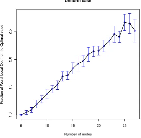
[image:27.595.175.414.246.480.2]Uniform case
Figure 6: Simulation results for the uniform case with 95% confidence intervals
simulations with 27 nodes, on average 217483 2-opt constraints were generated with an estimated standard deviation of 8081. The time for one iteration with 27 nodes is about 12790 seconds, more than 3.5 hours.
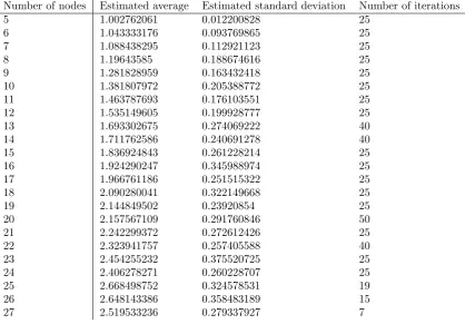
The results for this case are shown in Figure 6. This figure shows the average fraction found by the simulations along with a 95% confidence interval. The matching data is shown in Table 11.
Another matter to consider is if the simulation results agree with the theoretical results. This is
the experimental validation. For the uniform case we proved a bound ofOpnlog(n)in Section
3. We check this by looking at
[
WLOn
[
OPTn
p
nlog(n). (16)
HereWLO[n andOPT[n indicate the experimentally obtained values forWLOn andOPTn
respect-ively. We then compute the average value ofWLO[n/OPT[n which is indicated by the bar over this
Number of nodes Estimated average Estimated standard deviation Number of iterations
5 1.002762061 0.012200828 25
6 1.043333176 0.093769865 25
7 1.088438295 0.112921123 25
8 1.19643585 0.188674616 25
9 1.281828959 0.163432418 25
10 1.381807972 0.205388772 25
11 1.463787693 0.176103551 25
12 1.535149605 0.199928777 25
13 1.693302675 0.274069222 40
14 1.711762586 0.240691278 40
15 1.836924843 0.261228214 25
16 1.924290247 0.345988974 25
17 1.966761186 0.251515322 25
18 2.090280041 0.322149668 25
19 2.144849502 0.23920854 25
20 2.157567109 0.291760846 50
21 2.242299372 0.272612426 25
22 2.323941757 0.257405588 40
23 2.454255232 0.375520725 25
24 2.406278271 0.260228707 25
25 2.668498752 0.324578531 19
26 2.648143386 0.358483189 15
[image:28.595.93.512.109.400.2]27 2.519533236 0.279337927 7
Table 11: Simulation results for the uniform case
IfE[WLOn/OPTn] is inO( p
nlog(n)) we know that there is a positive constantM such that for large enough n we have |E[WLOn/OPTn]| ≤ M · |
p
nlog(n)|. In particular this means that for large enoughnwe have
E[WLOn/OPTn]
p
nlog(n) ≤M.
As such we expect the quantity in Equation (16) to eventually be a horizontal line. This would indicate that we have found a good bound. If the line would go down we divide by something that grows more quickly than the quantityWLOn/OPTn and we expect there to exist a beter bound.
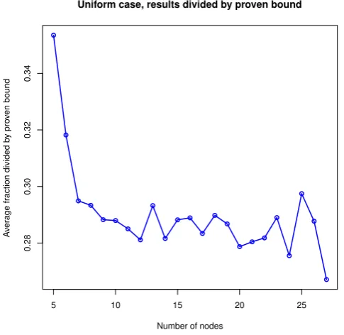
The results for the experiments are shown in Figure 7.
In this figure we do not see the results that we would expect to see. The line does not seem to converge to a horizontal line based on the data we collected. We discuss the significance of the experimental results in the next chapter.
6.5
Discrete distribution
5 10 15 20 25
0.28
0.30
0.32
0.34
Number of nodes
A
v
er
age fr
action divided b
y pro
v
en bound
[image:29.595.173.416.121.357.2]Uniform case, results divided by proven bound
Figure 7: Experimental validation for the uniform case
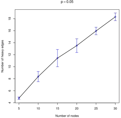
otherwise weight 2. We tested the following fixed values forp: 0.05, 0.1, 0.2, 0.5, 0.8, 0.9, 0.95, 0.99. Next to that we also tested the following expressions forp: 1/n, 1/√n and 1/log(n). Note that the theoretical results do not necessarily hold for these expressions, as it is only proven for fixed values ofp. The results of these simulations are presented in Figures 8 and 9 and Figures 13 to 21 in Appendix A. As in the uniform case we also want to see if we can validate the order bound proved theoretically. Our theoretical result showed that the number of heavy edges in the worst local optimum with respect to the 2-opt neighbourhood, E(#Heavy),∈O(log(n)) for a constant p. Hence we expect
#Heavy
log(n)
to eventually be (close to) a horizontal line. The results of this is shown in Figure 10. As before we do not clearly see the horizontal line we hope for. We do however notice the symmetry in the results aroundp= 0.5. The complete tables with results are shown in the appendix.
6.6
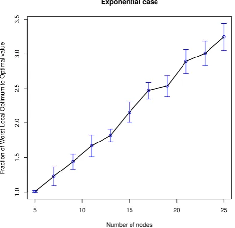
Exponential distribution
Finally we also want to experimentally check this exponential case. We again consider the fraction
WLOn/OPTn. For the generation of instances we also use Algorithm 6.3 using the Exponential
distribution with scale 1 for G. AIMMS has a function that generates random values drawn from the exponential distribution with lower bound land scale s: Exponential(l,s). We use
Exponential(0,1)to get a distribution with lower bound 0 and scale 1 and thus rate 1. We did
5 10 15 20 25 30
4
6
8
10
12
14
16
18
Number of nodes
Number of hea
vy edges
[image:30.595.173.415.140.375.2]p=0.05
Figure 8: Simulation results for the discrete case (p= 0.05) with 95% confidence intervals
5 10 15 20 25 30
4
6
8
10
12
14
Number of nodes
Number of hea
vy edges
p=0.1
[image:30.595.173.416.463.702.2]5 10 15 20 25 30
0
2
4
6
8
Number of nodes
A
v
er
age n
umber of hea
vy nodes divided b
y pro
ven bound
Discrete case, results divided by proven bound
[image:31.595.149.443.133.418.2]Values of p 0.99 0.95 0.9 0.8 0.5 0.2 0.1 0.05
Figure 10: Experimental validation for the discrete case
5 10 15 20 25
1.0
1.5
2.0
2.5
3.0
3.5
Number of nodes
Fr
action of W
orst Local Optim
um to Optimal v
alue
Exponential case
[image:31.595.175.415.484.716.2]5 10 15 20 25
0.12
0.14
0.16
0.18
0.20
0.22
Number of nodes
A
v
er
age fr
action divided b
y pro
v
en bound
[image:32.595.174.415.120.357.2]Exponential case, results divided by proven bound
Figure 12: Experimental validation for the exponential case
The theoretical result we proved says that E(WLOn/OPTn) ∈O q
nlog3(n)
. To validate we
again plot
WLOn
OPTn
q
nlog3(n)
and expect it to eventually be a horizontal line. The results of this are shown in Figure 12.
7
Discussion
In this section we discuss our results. We go through the different variants one by one and check how they fit with known results and whether the simulations support our results.
We first start by discussing the class of instances that we called generic on [0,1]. This part is both an extension and an improvement of the work done by Engels and Manthey (2009). We improved the upper bound on the average approximation ratio with respect to the 2-opt neighbourhood from O√n·(log(n))3/2toOpnlog(n). Furthermore, instead of just considering distances drawn
expended a previous result.
We now consider the case of discrete instances. In this thesis we used instances where each edge has a distance of 1 with probability p and 2 otherwise. Note that these distances are drawn at random and independently. For the discrete case we proved a result on the number of heavy edges in the worst local optimal solution. We show that in this case the number of heavy edges in the worst local optimum solution is inO(log(n)) ifpis a constant strictly between 0 and 1. As far as we are aware, this is the first average-case result on the approximation performance of 2-opt for discrete probability distributions. We also ran simulation for this case, for eight different values of pand for up to 30 nodes. For the validation for the constant values ofp, as shown in Figure 10 we see the data is quite consistent. We also recognize a symmetry around p= 0.5. Also, for p= 0.5 the line seems to be pretty much horizontal, indicating that we have found a good upper bound. Also the other values ofpallow for this as this are not decreasing and seem to level off over so slightly. However, before we make bold claims we must recall that the number of nodes used for these experiments is really quite low. Our results show behaviour that only needs to hold from a certain number of nodes onward. Hence we use caution in our claims. We still do feel that the experimental results support our theoretical results but experiments for larger instances are needed to make stronger claims.
Lastly we considered the instances where distances are drawn from a standard exponential dis-tribution. Because the exponential distribution does not have a bounded support, we had to use some more elaborate techniques. We assume wecan bound the distances and we choose the bound such that the probability if it being too low is extremely small. We have shown that the expected approximation ratio for the case with distances from the exponential distribution is
in O
q
nlog3(n)
. As with the discrete probability distributions, this is the first average-case
analysis of 2-opt with unbounded probability distributions, as far as we are aware. We also ran simulation to test our theoretical results. In this case we used up to 25 nodes. The experiment validation, found in Figure 12 shows a decreasing line which seems to level out. However, as before, because of the very limited number of nodes we have to cautiously approach the experiments. The data looks fairly consistent and we have an upper bound, a result we proved before. We cannot make claims regarding the quality of this upper bound as we would need more simulations with a higher number of nodes to get more useful results.
8
Conclusions
In this thesis we looked at the 2-opt heuristic for the traveling salesman problem. We have three main theoretical results, one of which is an improvement on earlier work and the other two are new results. Next to this we used simulations to experimentally check our bounds.
For the case with distances drawn randomly from the uniform distribution on [0,1] (and slightly more cases) we were able to show an upper bound on the expected approximation ratio of O(pnlog(n)). When the distances are either 1 with a fixed probability and 2 otherwise we were able to bound the number of edges with weight 2 in the worst locally optimal solution by O(log(n)). Lastly for distances drawn from the standard exponential distribution we were able to
showO
q
nlog3(n)
is an upper bound for the expected approximation ratio.
behaviour, whereas - in particular because finding worst local optima seems to be computationally difficult - our experiments are only for a relatively small number of nodes.
The results we presented in this thesis slightly improve the known upper bound on the performance of the 2-opt heuristic for the uniform distribution case. For the discrete case and the exponential case we presented new results. However, we do not know the exact bounds yet so there is certainly more work possible in this field, either by further improving the upper bounds or by showing lower bounds on the performance. In particular proving lower bounds seems to be quite difficult. We are not aware of any concrete techniques to prove lower bounds for this problem and thus this was kept out of this master thesis. This thesis only covers a very specific part of the fascinating field of the TSP, a problem that can appear easy at first sight, but also shows the limits of what we can achieve.
Acknowledgments
Bibliography
E.H.L. Aarts and J.K. Lenstra.Local Search in Combinatorial Optimization. Princeton University Press, 2003. ISBN 9780691115221. URLhttps://books.google.nl/books?id=NWghN9G7q9MC.
David L. Applegate, Robert E. Bixby, Vaˇsek Chv´atal, William Cook, Daniel G. Espinoza, Marcos Goycoolea, and Keld Helsgaun. Certification of an optimal TSP tour through 85,900 cities.
Operations Research Letters, 37(1):11 – 15, 2009. ISSN 0167-6377. doi: http://dx.doi.org/10. 1016/j.orl.2008.09.006.
D.L. Applegate, R.E. Bixby, V. Chv´atal, and W.J. Cook. The Traveling Salesman Problem: A Computational Study. Princeton Series in Applied Mathematics. Princeton University Press, 2011. ISBN 9781400841103. URLhttps://books.google.nl/books?id=zfIm94nNqPoC.
B. Chandra, H. Karloff, and C. Tovey. New results on the old k-opt algorithm for the traveling salesman problem. SIAM Journal on Computing, 28(6):1998–2029, 1999.
Georges A Croes. A method for solving traveling-salesman problems. Operations research, 6(6): 791–812, 1958.
C. Engels and B. Manthey. Average-case approximation ratio of the 2-opt algorithm for the TSP.
Operations Research Letters, 37(2):83–84, 2009. doi: 10.1016/j.orl.2008.12.002.
M. Englert, H. R¨oglin, and B. V¨ocking. Worst case and probabilistic analysis of the 2-opt algorithm for the TSP. Algorithmica, 68(1):190–264, 2014. doi: 10.1007/s00453-013-9801-4.
Lov K. Grover. Local search and the local structure of NP-complete problems.Operations Research Letters, 12(4):235 – 243, 1992. ISSN 0167-6377. doi: 10.1016/0167-6377(92)90049-9.
Michael Held and Richard M. Karp. A dynamic programming approach to sequencing problems.
Journal of the Society for Industrial and Applied Mathematics, 10(1):196–210, 1962. ISSN 03684245. URLhttp://www.jstor.org/stable/2098806.
David S Johnson and Lyle A McGeoch. The traveling salesman problem: A case study in local optimization. Local search in combinatorial optimization, 1:215–310, 1997.
Richard M. Karp. Reducibility among combinatorial problems. In Raymond E. Miller and James W. Thatcher, editors, Proc. of a Symp. on the Complexity of Computer Computations, pages 85–103. Plenum Press, 1972.
G¨ozde Kizilate¸s and Fidan Nuriyeva. On the Nearest Neighbor Algorithms for the Traveling Sales-man Problem, pages 111–118. Springer International Publishing, Heidelberg, 2013. ISBN 978-3-319-00951-3. doi: 10.1007/978-3-319-00951-3 11.
M. K¨unnemann and B. Manthey. Towards understanding the smoothed approximation ratio of the 2-opt heuristic. Lecture Notes in Computer Science (including subseries Lecture Notes in Artificial Intelligence and Lecture Notes in Bioinformatics), 9134:859–871, 2015. doi: 10.1007/ 978-3-662-47672-7 70.
B. Manthey and R. Veenstra. Smoothed analysis of the 2-opt heuristic for the TSP: Polynomial bounds for gaussian noise.Lecture Notes in Computer Science (including subseries Lecture Notes in Artificial Intelligence and Lecture Notes in Bioinformatics), 8283 LNCS:579–589, 2013. doi: 10.1007/978-3-642-45030-3 54.
List of Theorems
1.1 Definition (Traveling Salesman Problem (TSP)) . . . 4
1.2 Definition (Traveling Salesman Problem decision version (TSP-d)) . . . 5
3.5 Theorem (Result for general distribution) . . . 12
3.6 Corollary (Uniform distributions) . . . 13
3.7 Corollary (Standard uniform distribution) . . . 13
4.3 Theorem (Result for the discrete case) . . . 15
A
Graphical results for the discrete case
Most of the graphical results for variants of the discrete distribution have been moved this appendix because of the large amount of graphics. The descriptions for what is shown here can be found in Section 6.5.
5 10 15 20 25 30
4
6
8
10
Number of nodes
Number of hea
vy edges
[image:37.595.173.415.205.435.2]p=0.2
5 10 15 20 25 30
1.0
1.5
2.0
2.5
3.0
3.5
4.0
Number of nodes
Number of hea
vy edges
[image:38.595.174.415.137.374.2]p=0.5
Figure 14: Simulation results for the discrete case (p= 0.5) with 95% confidence intervals
5 10 15 20 25 30
4
6
8
10
Number of nodes
Number of hea
vy edges
p=0.8
[image:38.595.174.415.463.703.2]5 10 15 20 25 30
4
6
8
10
12
14
Number of nodes
Number of hea
vy edges
[image:39.595.172.415.139.375.2]p=0.9
Figure 16: Simulation results for the discrete case (p= 0.9) with 95% confidence intervals
5 10 15 20 25 30
4
6
8
10
12
14
16
18
Number of nodes
Number of hea
vy edges
p=0.95
[image:39.595.174.415.463.703.2]5 10 15 20 25 30
5
10
15
20
25
Number of nodes
Number of hea
vy edges
[image:40.595.173.415.140.375.2]p=0.99
Figure 18: Simulation results for the discrete case (p= 0.99) with 95% confidence intervals
5 10 15 20 25 30
5
10
15
20
Number of nodes
Number of hea
vy edges
p=1 n
[image:40.595.174.416.456.702.2]