Discharge and location dependency of calibrated main channel roughness: case study on the river Waal and IJssel

(1)

DISCHARGE AND LOCATION

DEPENDENCY OF CALIBRATED

MAIN CHANNEL ROUGHNESS:

CASE STUDY ON THE RIVER WAAL

AND IJSSEL

.

Technical report

Author

(2)

(3)

DISCHARGE

AND

LOCATION

DEPENDENCY

OF

CALIBRATED MAIN CHANNEL ROUGHNESS: CASE

STUDY ON THE RIVER WAAL AND IJSSEL

Technical report

This report is a part of a graduation research

Adjacent to this report a conference paper has been written

Delft, Januari 2018

Author

Boyan Domhof BSc

Co-authors

Ir. K.D. Berends (University of Twente) Dr. ir. A. Spruyt (Deltares)

Dr. J.J. Warmink (University of Twente)

(4)

Abstract

To accurately predict water levels, river models require appropriate description of hydraulic roughness. In most calibration studies of hydrodynamic models the hydraulic roughness coefficient is calibrated because it is the most uncertain parameter (Bates et al., 2004; Hall et al., 2005; Pappenberger et al., 2005; Refsgaard et al., 2006; Vidal et al., 2007; Warmink et al., 2011). The roughness increases as river dunes grow with increasing discharge and is dependent on differences in channel width, bed level and bed sediment. Therefore, we hypothesize that the calibrated main channel roughness coefficient is most sensitive to the discharge and location in longitudinal direction of the river. The calibration study of Warmink et al. (2007) confirms this hypothesis. However, the study of Warmink et al. (2007) does not explain why the calibrated roughness varies along the longitudinal direction of the river and the discharge stages. The main objective in this study is to investigate the location and discharge dependency on the main channel roughness the River Waal and IJssel by calibration. Validation is performed to check if the calibrated roughness also results in accurate water level predictions. The conclusions of this study can be used to improve future calibration studies.

The main channel roughness is calibrated using the Manning roughness formula in the 1D hydrody-namic models of the River Waal for the winters of 1995 and 2011 and IJssel for the winter of 1995 in the Netherlands. The location dependency in the longitudinal direction of the river is modelled using a vary-ing number of roughness trajectories. The discharge dependency is modelled usvary-ing a varyvary-ing number of discharge levels. Calibration is performed automatically with the software package OpenDA using the DuD algorithm and a weighted non-linear least squares objective function. Validation is performed using a slightly adapted RMSE criterion.

Results show that the calibrated roughness is mainly sensitive to discharge. Especially the transition from bankfull to flood stage, the effect of the modelled summer dike and the overestimation of bankover-flow in sharp bends are important features to consider in the calibration as it produces better water level predictions. Especially the effect of the modelled summer dike on the calibrated roughness is significant. The optimum number of discharge levels ranges between 4 and 8 discharge levels.

(5)

1 Introduction

1.1 Background

Hydrodynamic river models are used to predict water levels along the river and support decision making in river management. The models are used to monitor the river and to study the effects of measures in the river to decrease the risk of flooding in high water situations and prevent drought in low water situations. Therefore, the model predictions need to be sufficiently accurate. Insufficiently accurate predictions can for example lead to the construction of dikes which are too low which in turn can lead to major damages and casualties in case of flooding.

Hydrodynamic models are calibrated and validated to increase accuracy. Calibration involves min-imizing the errors between predicted and observed water levels by altering model parameters for a specific situation. Validation involves verifying if the calibrated model parameters also produce small to no errors between predicted and observated water levels in different situations. In most calibration studies of hydrodynamic models the hydraulic roughness coefficient is calibrated because it is the most uncertain parameter (Bates et al., 2004; Hall et al., 2005; Pappenberger et al., 2005; Refsgaard et al., 2006; Vidal et al., 2007; Warmink et al., 2011). Furthermore, this coefficient is often treated as a dustbin parameter which can compensate for all kinds of model errors, for example simplifying the river bathymetry into a limited number of cross-sections (Morvan et al., 2008 as cited in Warmink, 2011).

Along the longitudinal direction of the river differences in main channel and floodplain width, bed level and bed sediment can for example lead to varying calibrated roughness values. The floodplain vegetation influences the roughness during flood discharge stage. Moreover, as discharge increases, river dunes grow. This is turn increases the bed roughness (Julien et al., 2002). Therefore, it is hypothe-sized that the calibrated hydraulic roughness is mostly sensitive to discharge and location in longitudinal direction of the river. The calibration study of Warmink et al. (2007) confirms this hypothesis. However, this study does not explain why the calibrated roughness varies along the longitudinal direction of the river and the discharge stages. Our study provides explanations why these variations occur and whether location or discharge dependency is most sensitive. We only focus on the River Waal and IJssel in The Netherlands.

1.2 Objective

(7)

1.3 Scope

In this study we investigate the main channel hydraulic roughness parameters for 1D hydrodynamic river models of large lowland normalized rivers used for water level predictions. The choice for 1D models is based on the shorter calibration times compared to the computational times of 2D (or even 3D) models. We only calibrate the main channel hydraulic roughness parameters. The choice for models of large lowland normalized rivers is based on the availability of and experience with these models at Deltares. The Manning roughness formula is used for the main channel roughness coefficient because it is better suited in the use of compound channels (Huthoff & Augustijn, 2004).

1.4 Contributions

The main part of this study is performed by Boyan Domhof as part of his graduation project. Much input is given by Aukje Spruyt and Koen Berends. Jord Warmink and Suzanne Hulscher independently reviewed the research.

1.5 Report outline

(8)

2 Method

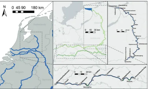
2.1 Study area

2.1.1 Waal

The Waal is a tributary of the River Rhine. It is relatively straigth and has consistent main channel width which doubles as the river approaches the sea. A schematization of the Waal river model with its observation stations is presented in Figure 2.1. The Waal river starts at river chainage 867 km and ends at 961 km. Note: the river chainage in the models is shorter, namely the river ends at 959.48 km. Figures therefore only present the river chainage from 867 to 959.48 km. The Waal has 7 water level observation stations of which 5 stations can be used in the calibration:

1. Pannerdensch Kop (PK); 2. Nijmegenhaven (NH);

3. Dodewaard (DW) (constructed after 1995); 4. TielWaal (TW);

5. Zaltbommel (ZB); 6. Vuren (Vu);

7. Hardinxveld (HV) (adjusted location of Werkendam in model, cannot be used in calibration because it is the most downstream location).

The Waal has three important features to consider, namely two armoured bed layers and submerged groynes in certain river bends to prevent erosion of the sandy bed in the outer bend. An armoured bed layer is present in the bend near Nijmegen and has been constructed in 1988. In the bend at Sint Andries an armoured bed layer has been constructed too, in 1999. In the bend near Erlecom submerged groynes have been constructed in 1996. These features have a large impact on the roughness and therefore on the water levels. Berends (2013) describes a way to deal with these layers in the calibration of the Waal model, which is summarized in Appendix A.

2.1.2 IJssel

(9)

1. IJsselkop (IJK);

2. Westervoort (WV) (constructed after 1995); 3. De Steeg (DeS) (constructed after 1995); 4. Doesburgbrug (DB);

5. Zutphennoord (Zut);

6. Eefebeneden (EB) (constructed after 1995); 7. Deventer (DV) (constructed after 1995); 8. Olst (Olst);

9. Wijhe (Wij) (constructed after 1995); 10. Katerveer (KV);

11. Kampenbovenhaven (KH);

[image:9.595.50.552.279.582.2]

12. Keteldiep/Kattendiep (Kdiep) (cannot be used in calibration because it is the most downstream location).

(10)

2.2 Study cases

Three study cases are performed:

Waal 1995 Calibration on Waal 1995 model and validation on Waal 1993 and 2011 models

IJssel 1995 Calibration on IJssel 1995 model and validation on IJssel 2011 model

Waal 2011 Calibration on Waal 2011 model and validation on Waal 2015 model

2.2.1 Waal 1995

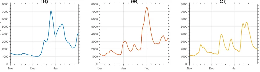
[image:10.595.77.524.347.472.2]

The discharge wave of 1995 is used for the calibration. This discharge wave is the highest recorded in the Netherlands in recent history and thus provides a large range of discharge levels to calibrate on. The discharge waves of 1993 and 2011 are used for validation. The discharge waves are illustrated in Figure 2.2. The time periods for the three different waves are the following:

1993 (validation) 01/11/1993 00:00 - 31/01/1994 23:00

1995 (calibration) 01/12/1994 00:00 - 28/02/1995 23:00

2011 (validation) 01/11/2010 00:00 - 31/01/2011 23:00

Nov Dec Jan

0 1000 2000 3000 4000 5000 6000 7000 8000

Discharge [m

3/s]

1993

Dec Jan Feb

0 1000 2000 3000 4000 5000 6000 7000 8000

1995

Nov Dec Jan

0 1000 2000 3000 4000 5000 6000 7000 8000

2011

Figure 2.2: Discharge waves of 1993, 1995 and 2011 at Pannerdensch Kop

2.2.2 IJssel 1995

The discharge in the IJssel is a small fraction of the Waal. The discharge wave of 1995 is used for calibration. The discharge waves of 1993 and 2011 are used for validation. The discharge waves are illustrated in Figure 2.3 and the following time periods apply:

1993 (validation) 01/11/1993 00:00 - 31/01/1994 23:00

1995 (calibration) 01/12/1994 00:00 - 28/02/1995 23:00

(11)

Nov Dec Jan 0

500 1000 1500 2000

Discharge [m

3/s]

1993

Dec Jan Feb

0 500 1000 1500 2000

1995

Nov Dec Jan

0 500 1000 1500 2000

2011

Figure 2.3: Discharge waves of 1993, 1995 and 2011 at IJsselkop

2.2.3 Waal 2011

Both the Waal 2011 and 2015 models are more recent and include some measures of the ’Room for the River’-project (especially the 2015 model). Figure 2.4 presents the discharge waves of 2011 and 2015 of the Waal. The time periods for the two different waves are the following:

2011 (calibration) 01/11/2010 00:00 - 31/01/2011 23:00

2015 (validation) 01/11/2015 00:00 - 31/03/2016 23:00

Nov Dec Jan

0 2000 4000 6000 8000

Discharge [m

3/s]

2011

Nov Dec Jan Feb Mar

0 2000 4000 6000 8000

2015

Figure 2.4: Discharge waves of 2011 and 2015 at Pannerdensch Kop

Note: the discharge wave data of 2015 at Pannerdensch Kop has not been corrected for volumetric differences as was done for the 1993, 1995 and 2011 discharge waves.

2.3 Models

Four different versions of the Dutch Rhine-model (of which the Waal and IJssel are part) are used following the presented study cases:

1. j93 5-v4 (1993) 2. j95 5-v4 (1995) 3. j11 5-v3 (2011) 4. j15 5-v2 (2015)

(12)

2.4 Location dependency

To investigate the location dependency of the main channel roughness, three different situations (of which the Waal 1995 calibration is illustrated in Figure 2.5) are calibrated:

1. Whole time-period of discharge wave; 2. Discharge level in bankfull stage; 3. Discharge level in flood stage.

01/12 01/01 01/02

0 2000 4000 6000 8000

Discharge [m

3/s]

Whole discharge wave

01/12 01/01 01/02

0 2000 4000 6000 8000

Bankfull stage

1850 ± 150

01/12 01/01 01/02

0 2000 4000 6000 8000

Flood stage

7550 ± 150

Figure 2.5: Three calibration cases illustrated: using 1) whole discharge wave, 2) a discharge level of 1850±150

m3_{/s on only the first and lowest discharge peak (bankfull stage) and 3) a discharge level of 7550}_{±150 m}3_{/s on}

only the fourth and highest discharge peak (flood stage)

Note: Because the discharge wave in the IJssel greatly changes as it progresses more downstream (i.e. due to diffusion of the wave and large lateral discharge sources like the Twentekanaal), the discharge levels are changed in size and height according to the progression of the wave.

2.4.1 Calibration routine

All the observation data are taken into account in the calibration, because we want to capture as much of the river behaviour as possible. The roughness trajectory configuration for N number of trajectories is presented in Table 2.1. The trajectory lengths are roughly of equal length. Otherwise, no calibration takes place indicated by n.a. in the table.

Note: Also calibrations on 2D WAQUA results, used as a representation of the observation data, were performed for the Waal 1995 case. In these calibrations we could increase the number of roughness trajectories above the number of existing roughness trajectories. However, these calibration proved to be unsuccesful as the calibrated 1D model was too similar to the 2D model.

Table 2.1: Roughness trajectory configuration for varying number of trajectories and for the Waal 1995, IJssel 1995 and Waal 2011 cases

N traj. Waal 1995 IJssel 1995 Waal 2011

1 PK-HV IJK-Kdiep PK-HV

2 PK-TW, TW-HV IJK-Olst, Olst-Kdiep PK-TW, TW-HV

3 n.a. IJK-Zut, Zut-KV, KV-Kdiep PK-DW, DW-ZB, ZB-HV

4 PK-NH, NH-TW, TW-ZB,

ZB-HV n.a. n.a.

5 PK-NH, NH-TW, TW-ZB,

ZB-Vu, Vu-HV

IJK-DB, DB-Zut, Zut-Olst, Olst-KV, KV-Kdiep

PK-NH, NH-DW, DW-TW, TW-ZB, ZB-HV

6 n.a. IJK-DB, DB-Zut, Zut-Olst,

Olst-KV, KV-KH, KH-Kdiep

(13)

2.5 Discharge dependency

In each calibration case the five (Waal 1995) or six (IJssel 1995 and Waal 2011) existing roughness trajectories are calibrated with a varying number of discharge levels. Four scenarios are distinquished in applying discharge levels:

Scenario 1: peaks Based on discharge peaks

Scenario 2: valleys Based on discharge valleys

Scenario 3: peaks and valleys Based on both discharge peaks and valleys

Scenario 4: robust method Based on dividing the discharge wave inN equally-spaced dis-charge levels

We refer to scenarios 1, 2 and 3 as the method with discharge levels which are more or less determined by a constant discharge for a longer period of time, ”constant discharge levels method”. It ensures that the calibration is focused on one discharge value without being dominated by the water level errors due to the ”rising” and ”falling” parts (i.e. steep incline/decline before/after the peak/valley) of the discharge wave. Calibration scenarios 1, 2 and 3 are not performed for the IJssel 1995 and Waal 2011 cases.

Scenarios 1, 2 and 3, however, largely depend on subjective choices (e.g. which peaks and valleys are to be calibrated, which discharge wave is going to be used, how big is the window around the discharge levels). To avoid making these choices and therefore have a more objective method, we present a robust method where the discharge wave is divided into N equal-spaced discharge levels, from (roughly) the minimum to the maximum discharge of the wave, which are calibrated in one run. In this case, two choices remain, namely which discharge wave and how many discharge levels are to be used in calibration. We refer to this scenario as the ”robust method” as this method can be applied to any discharge wave irrespectively of the shape, length and height of the discharge wave. The discharge dependency calibrations of the IJssel 1995 and Waal 2011 are only performed with the robust method.

2.5.1 Scenario 1-3: Constant discharge levels method

Discharge levels

Figure 2.6 illustrates scenarios 1, 2 and 3 for the Waal 1995 calibration. In the figure only the color-highlighted parts of the discharge wave are calibrated. Each discharge level is placed roughly on the bottom of the valley or top of the peak with a standard window of 150 m3_{/s. The latter means there is}

a bandwith of plus and minus 150 m3_{/s around the set discharge level. When the discharge windows}

of peaks or valleys overlap, they are defined as one level, as, for example, can be seen for level 1750

±150 m3_{/s in the second subplot of the figure.}

Calibration routine

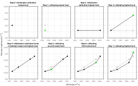
The three scenarios are calibrated using a standard calibration procedure, as illustrated in Figure 2.7. In this procedure, we start with calibrating the lowest discharge level and move up to the highest discharge level. The choice of starting with the lowest discharge level is because at this point it is in the bankfull stage. Therefore, only the effects of the main channel are calibrated into the main channel roughness. Table 2.2 presents the levels which are calibrated forN number of discharge levels for each of three scenarios. The calibration procedure is as follows (and graphically illustrated in Figure 2.7):

(14)

01/12 01/01 01/02 0

1000 2000 3000 4000 5000 6000 7000 8000

Discharge [m

3/s]

Scenario 1: peaks

1850 ± 150

2600 ± 150 3000 ± 150

3750 ± 150 7550 ± 150

01/12 01/01 01/02

Scenario 2: valleys

1250 ± 150 1750 ± 150

2700 ± 150 3050 ± 150

01/12 01/01 01/02

Scenario 3: peaks and valleys

1250 ± 150

1750 ± 150 2650 ± 150

3000 ± 150

[image:14.595.51.546.70.258.2]

3750 ± 150 7550 ± 150

Figure 2.6: Scenarios 1, 2 and 3 illustrated on the 1995 discharge wave

Table 2.2: Discharge levels which are calibrated forN number of discharge levels for scenario 1, 2 and 3 for Waal

1995 calibration

# of levels Scenario 1: peaks Scenario 2: valleys Scenario 3: peaks and valleys

2 Q1850 Q7550 Q1250 Q3050 Q1250 Q7550

3 Q1850 Q3000 Q7550 Q1250 Q2700 Q3050 Q1250 Q2650 Q7550

4 Q1850 Q2600 Q3750 Q7550 Q1250 Q1750 Q2700 Q3050 Q1250 Q2650 Q3750 Q7550

5 Q1850 Q2600 Q3000 Q3750 Q7550 n.a. n.a.

6 n.a. n.a. Q1250 Q1750 Q2650 Q3000 Q3750 Q7550

roughness of the lowest discharge level is used as the initial roughness for the roughness calibra-tion of the highest discharge level. This will result in a linear roughness-discharge relacalibra-tion.

N >2levels In the next step, the roughness discharge function, obtained in the previous two levels

calibration case, is used as the initial roughness estimation. Depending on theN number of levels, we interpolate the initial roughness for the given discharge level height on this linear roughness discharge function. Next, we calibrate the roughness starting with the second lowest discharge level. After that, we calibrate the next lowest discharge level, till we have calibrated the highest discharge level as the last level.

2.5.2 Scenario 4: Robust method

Discharge levels

Scenario 4 involves using the robust method which has minimal (subjective) choices to be made and can be used for any discharge wave. The discharge wave is divided intoN equal-spaced discharge levels from (roughly) the minimum to (roughly) the maximum discharge of the wave withN = [2,3,4,6,8,12]. ForN = 2the minimum and maximum discharge (thus 1000 and 8000 m3_{/s) are choosen as the two}

[image:14.595.54.542.321.422.2]

(15)

Discharge [m3/s]

Manning roughness [s/m

1/3

]

1000 1500 2000 2500 3000 0.02

0.025 0.03 0.035 0.04 0.045

Step 0: initialisation calibration lowest level

1000 1500 2000 2500 3000

Step 1: calibrating lowest level

1000 1500 2000 2500 3000

Step 2: initialisation calibration highest level

1000 1500 2000 2500 3000

Step 3: calibrating highest level

1000 1500 2000 2500 3000 0.02

0.025 0.03 0.035 0.04 0.045

Step 4: initialisation calibration levels in between lowest and highest level

1000 1500 2000 2500 3000

Step 5: calibrating second lowest level

1000 1500 2000 2500 3000

Step 6: calibrating third lowest level

Calibration procedure for 4 levels, scenario 2: valleys

1000 1500 2000 2500 3000

[image:15.595.70.527.78.364.2]

Step 7: calibrating highest level

Figure 2.7: Example of the calibration procedure, illustrated using 4 discharge levels for scenario 2: valleys on the Waal 1995 discharge wave. A green dot indicates a newly calibrated discharge level.

Table 2.3: Minimum and maximum discharge levels (in m3_{/s) for robust method for Waal 1995, IJssel 1995 and Waal}

2011 cases

Case Minimum Maximum

Waal 1995 1000 8000

IJssel 1995 200 1900

Waal 2011 750 600

Calibration routine

OpenDA provides the ability to calibrate all the discharge levels in one calibration run. During this ”everything-at-once”-run we calibrate on the whole time period of the discharge wave. Due to this ap-proach it is expected that OpenDA needs more iterations to find a solution for the calibration problem. Therefore, the maximum number of outer iterationsN1is increased to 100 and the maximum number of

inner iterationsN2to 10 compared to the standard calibration options as presented in Table 2.4.

First forN = 2, both the levels at the minimum and maximum are calibrated in one run using the standard initial roughness of n = 0.03 s/m1/3_{. For} _{N >} ₂_{, we first generate an initial estimate of the}

[image:15.595.217.378.439.498.2]

(16)

2.6 Calibration method

OpenDA (OpenDA, 2015) is used to calibrate the 1D hydrodynamic models using a weighted non-linear least squares objective function and the DuD-algorithm (Ralston & Jennricht, 1978). The standard calibration options are stated in Table 2.4. The calibration is based on water levels. Windows around a discharge level can be used to limit the time period of the water level data to be used in calibration (e.g. only calibrating the top of a discharge peak). The initial roughness before calibration is set at Manning 0.03 s/m1/3 _{corresponding to a sandy dune bed (Julien, 2002). In each calibration case, the}

trajectory roughness is determined as uniform along the whole trajectory. Finally, the first three days of the discharge wave are not taken into account for the calibration to remove any remaining model initialization errors.

2.7 Performance criteria

We choose to use the Root Mean Square Error (RMSE) function to evaluate the performance of the model in the calibration and validation cases due to the mathematical similarity with the used objective function (i.e. weighted nonlinear least squares [as shown in Table 2.4]) in OpenDA:

RM SE=

v u u t

1

k·l k X

i=1

l X

j=1

γi,j·(yi,j−yˆi,j)

2

(2.1)

withydenoting the simulated water levels,yˆdenoting the observed water levels,γdenoting a weighting factor, l denoting the number of observed water levels of one observation location andkdenoting the number of observation stations. In case of k = 1, only the RMSE of one observation station is calcu-lated. When multiple observation stations are taken into account, thusk >1, the number oflobserved water levels should be equal for allkobservation stations to ensure each residual weighs equally in the calculated RMSE. The first three days of water level data is discarded following the same choice in the calibration.

(17)

T ab le 2.4: Calibr atio n options that are used in this study . yi j denotes the obser v ated w ater le v el and ˆ yij ( θ ) the sim ulated w ater le v el for a giv en time j with l the n umber of time instances , a giv en obser v ation location i with k the n umber of locations and θ denoting a set of calibr ation par ameters . Description Form ula V alue Notes Calibration algorithm DuD (Doesn’t use Der iv ativ es) The choice of the DuD calibr ation algor ithm is based on its ro-b ustness and efficiency on non-linear functions (e .g. large-scale 1D h ydrodynamic riv er models) and con v erges the quic k est in compar ison to the simple x and P o w ell’ s method (Schw anenberg et al., 2011; P ost, 2012; Mulder , 2014). Objective function W eighted nonlinear least squares Q ( θ ) Q ( θ ) = 1 2 k X i =1 l X j =1 W i ( yij − ˆ yij ( θ )) 2 W i = 1 /σ 2 i with σi the measu rement uncer tainty of each obser v a-tion station which is equal to 0.01 m for each obser v ation station in the W aal and IJssel Stopping criteria Maxim um n umber of outer iter ations N1 20 An outer iter ation is par t of the calibr ation routine . Maxim um n umber of outer iter ations N2 5 An outer iter ation is par t of the calibr ation routine . Maxim um absolute objec-tiv e diff erence T1 | Q ( θnew ) − Q ( θ0 ) | < T1 1.0 Maxim um relativ e objec-tiv e diff erence T2 | Q ( θnew ) − Q ( θ0 ) | | Q ( θ0 ) | < T2 0.0001 Maxim um relativ e lin-ear iz ed objectiv e diff er-ence T3 |

˜_Q(

θnew

)

−

˜_Q(

θ0

)|

|

˜_Q(

(18)

3 Results: calibration

3.1 Location dependency calibrated roughness values

Figures 3.1, 3.2 and 3.3 show the calibrated roughness for the Waal 1995, IJssel 1995 and Waal 2011 models for a varying number of roughness trajectories. Overall, the calibrated values are fairly constant along the whole river length. More large deviations in calibrated roughness values between the three different cases (i.e. whole discharge wave, bankfull and flood discharge level) occur at the downstream boundary. This can be attributed to an insufficiently correct boundary condition. The backwater effect occuring because of the boundary condition does not predict the water levels correctly at the observation stations influenced by the backwater effect. The calibration compensates for this by adjusting the rough-ness. For the Waal models, the roughness is lowered for the bankfull stage and increased for the flood stage. This effect is not present in the IJssel model, where the roughness at the downstream boundary is roughly the same for both bankfull and flood stage cases. The difference in roughness for the Waal models can be attributed to a changing backwater (i.e. from an M1 to an M2 curve (Chow, 1959, p.226)). In the Waal models a roughness increase at Dodewaard/TielWaal (between 901 and 933 km) can be seen. It is unknown why this happens.

River chainage [km]

1/3

]

0.02 0.03 0.04

0.05 # of traj. = 1 # of traj. = 2

860 870 880 890 900 910 920 930 940 950 960 0.02 0.03 0.04

0.05 # of traj. = 4

waal_j95_calibrated_wholewave, waal_j95_calibrated_q1850 and waal_j95_calibrated_q7550

860 870 880 890 900 910 920 930 940 950 960

# of traj. = 5 wholewave q1850 q7550

Figure 3.1: Calibrated roughness of the Waal for whole discharge wave, with a 1850 m3/s discharge level (bankfull

stage) and with a 7550 m3/s discharge level (flood stage) for 1995 discharge wave for varying number of roughness

trajectories. Dotted black lines show the division intoN number of trajectories, grey dots above x-axis show the

(19)

River chainage [km]

1/3

] 0.02 0.03 0.04

0.05 # of traj. = 1 # of traj. = 2

0.02 0.03 0.04

0.05 # of traj. = 3

880 900

920 940

960 980

1000

# of traj. = 5

ijssel_j95_calibrated_wholewave, ijssel_j95_calibrated_q400, ijssel_j95_calibrated_q1800

880 900

920 940

960 980

1000 0.02 0.03 0.04

0.05 # of traj. = 6

[image:19.595.54.545.83.287.2]

wholewave q400 q1800

Figure 3.2: Calibrated roughness of the IJssel for whole discharge wave, with a 400 m3_{/s discharge level (bankfull}

stage) and with a 1800 m3/s discharge level (flood stage) for 1995 discharge wave for varying number of roughness

observation locations

River chainage [km]

1/3

] _0.02 0.03 0.04

0.05 # of traj. = 1 # of traj. = 2

0.02 0.03 0.04

0.05 # of traj. = 3

860 870 880 890 900 910 920 930 940 950 960

# of traj. = 5 waal_j11_calibrated_wholewave, waal_j11_calibrated_q1350, waal_j11_calibrated_q5500

860 870 880 890 900 910 920 930 940 950 960 0.02 0.03 0.04

0.05 # of traj. = 6

Figure 3.3: Calibrated roughness of the Waal for whole discharge wave, with a 1350 m3/s discharge level (bankfull

stage) and with a 5500 m3_{/s discharge level (flood stage) for 2011 discharge wave for varying number of roughness}

observation locations. The small roughness increases around 874, 883 and 926 km are due to respectively the submerged groynes at Erlecom and the armoured bed layers at Nijmegen and Sint Andries

[image:19.595.50.545.370.577.2]

(20)

large cross-sectional profile with large storage areas in the bends (illustrated in Figure 3.5), but this is insufficient. The calibration then ultimately solves this problem by lowering the roughness.

8 10 12 14

Water level [m]

IJsselkop

21/01 31/01 10/02

-0.5 0 0.5

Simulated minus

obsversation water level [m]

7 8 9 10

11 Doesburgbrug

21/01 31/01 10/02

-0.5 0 0.5

5 6 7 8

9 Zutphennoord

21/01 31/01 10/02

-0.5 0 0.5

2 4 6

8 Olst

21/01 31/01 10/02

-0.5 0 0.5

0 1 2 3

4 Katerveer

21/01 31/01 10/02

-0.5 0 0.5

-1 0 1 2

3 Kampenbovenhaven Obs SOBEK (bankfull stage calibrated)

21/01 31/01 10/02

[image:20.595.53.544.114.269.2]

-0.5 0 0.5

Figure 3.4: Water level overestimation in the bends of the IJssel for the flood stage of 1995. The water levels are largely overestimated at Doesburgbrug and Zutphennoord. The water level at Olst is nor under- or overestimated

Rhederlaag

Doesburgbrug

[image:20.595.117.472.321.533.2]

(21)

3.2 Discharge dependency calibrated roughness-discharge

func-tions

Only the robust method results (i.e. scenario 4) are considered here. The calibrated roughness of scenarios 1, 2 and 3 for the Waal can be found in Appendix C. A calibration with the robust method for the 2D WAQUA 1995 Waal model is performed too using six discharge levels. These calibration results can be found in Appendix E.

Figures 3.6, 3.7 and 3.8 show the calibrated roughness-discharge functions for a varying number of roughness trajectories. The roughness functions for all three models show overall increasing roughness with discharge. This is not true for the trajectories DB-Zut and Zut-Olst for the IJssel model due to overestimation of the water levels in the river bends (see previous section for more information). When adding more discharge levels, more details in the roughness-discharge functions appear. The most prominent details are the roughness increase at lower discharges after which a roughness decrease occurs to finally end in a roughness peak at higher discharges.

Discharge level [m3_/s]

1/3

]

2000 4000 6000 8000 0.02

0.025 0.03 0.035 0.04 0.045

0.05 Traject PK-NH

2000 4000 6000 8000 Traject NH-TW

2000 4000 6000 8000 Traject TW-ZB

2000 4000 6000 8000 Traject ZB-Vu

2000 4000 6000 8000 Traject Vu-HV waal_j95_calibrated_robust_method

[image:21.595.50.545.477.589.2]

# of levels = 2 # of levels = 3 # of levels = 4 # of levels = 6 # of levels = 8 # of levels = 12

Figure 3.6: Calibrated roughness-discharge functions of the Waal for 1995 discharge wave for varying number of discharge levels based on the robust method

1/3

]

500 1000 1500 0.02

0.025 0.03 0.035 0.04 0.045

0.05 Traject IJK-DB

500 1000 1500

Traject DB-Zut

500 1000 1500

Traject Zut-Olst

500 1000 1500

Traject Olst-KV

500 1000 1500

Traject KV-KH

500 1000 1500

Traject KH-Kdiep

ijssel_j95_calibrated_robust_method

(22)

1/3

]

2000 4000 6000 0.02

0.025 0.03 0.035 0.04 0.045

2000 4000 6000

Traject NH-DW

2000 4000 6000

Traject DW-TW

2000 4000 6000

Traject TW-ZB

2000 4000 6000

Traject ZB-Vu

2000 4000 6000

Traject Vu-HV

waal_j11_calibrated_robust_method

[image:22.595.48.545.75.186.2]

Figure 3.8: Calibrated roughness-discharge functions of the Waal for 2011 discharge wave for varying number of discharge levels based on the robust method

The roughness increase at lower discharges can be attributed to the growth of river dunes. As these bedforms grow, the roughness also grows (Julien et al., 2002; Wilbers & Ten Brinke, 2003). This growth could also explain why the calibrated roughness increases overall with discharge.

The roughness decrease around 4000 m3_{/s for the Waal and 800 m}3_{/s for the IJssel after the increase}

can be attributed to the transition from bankfull to flood stage. When the water level starts to flow into the floodplain, the total wetted perimeter suddenly increases whereas the total wetted area remains fairly constant. This results in a sudden decrease in the hydraulic radius and this in turn leads to a lower compound roughness (see Figure 3.9). However, as the calibrated roughness still decreases, it is assumed that the lowering of the compound roughness is not sufficient enough to accurately predict the water level at that stage. The discharge at which this transition occurs depends on the roughness at lower discharges. A high roughness at lower discharges results in a higher water level which in turn leads to a more early flow into the floodplain.

Figure 3.9: Water level and hydraulic radius as a function of the discharge at Zaltbommel for 2 discharge levels. The cross-sectional profile is plotted too. The box in the left plot indicate the drop and recovery of the total hydraulic radius

[image:22.595.96.505.430.557.2]

(23)

Figure 3.10: Predicted and observed water level at Zaltbommel. Discrepancy between predicted and observed wa-ter level is more concentrated on rising limb for 2 levels. Roughness increase at 6 levels minimizes total discrepancy for both rising and falling limb

The discrepancy is centered around one specific discharge due to the way the overflow over the summer dike is modelled (Deltares, 2015, p.90). A discrepancy on the falling limb of the discharge peak also starts to form but but across the whole range of the peak. This is also a result of how the flow of the stored water behind the summer dike back into the main channel is modelled. In the end, we see a large discrepancy on the rising limb of the discharge peak for a specific discharge whereas a more spread out discrepancy on the falling limb of the peak occurs. The calibration favors the larger discrepancy on the rising limb over the more spread out discrepancy on the falling limb and ultimately increases the roughness at a specific discharge level to minimize the total error between predicted and observed water levels. The roughness peak is less apparent in the calibrated roughness of the Waal 2011 model because multiple moderately high discharge peaks occur in this discharge wave leading to a more spread out calibration result.

During the investigation of the effect of the modelled summer dike, we found that the flow area of the modelled summer dike is in most cross-sections in the used models higher than the total area. These areas are calculated by the WAQ2PROF method. Physically a larger flow area than the total area is not possible but SOBEK ignores this by calculating the effect of the flow and total area seperately. Therefore, the flow area is mostly overestimated leading to a very high roughness peak. Although calibration solves this problem, still it is not ideal. A calibration is performed with six discharge levels on the Waal 1995 model where the flow area is manually limited to the total area. Furthermore, a calibration without the modelled summer dike is performed too. Figure 3.11 shows the calibrated roughness-functions of these two calibrations compared to the case without adjustment to the modelled summer dike. The figure shows that the modelled summer dike has a very large impact on the calibrated roughness at higher discharges. It is advised to investigate how this impact translates to the accuracy of the predicted water levels.

Discharge level [m3/s]

1/3

]

2000 4000 6000 8000 0.02

0.025 0.03 0.035 0.04 0.045

2000 4000 6000 8000 Traject NH-TW

2000 4000 6000 8000 Traject TW-ZB

2000 4000 6000 8000 Traject ZB-Vu waal_j95_calibrated_roughness_6_levels_5_traj_summerdike_option

2000 4000 6000 8000 Traject Vu-HV

[image:23.595.195.402.71.193.2]

Summer dike default Flow area corrected Summerdike off

(24)

4 Results: validation

4.1 Location dependency model performance

Figures 4.1, 4.2 and 4.3 present the validation of the calibration on the Waal 1995, IJssel 1995 and Waal 2011 models for a varying number of roughness trajectories. All validation cases show the worst model performance when calibrating on a discharge level in the flood stage (i.e. highest discharge peak). This is because only during the highest discharge peak the water levels get simulated correctly. When calibrating on a discharge level in the bankfull stage (i.e. lowest discharge peak or deepest discharge valley), then model performance is much better. However, taken the whole discharge wave into account in the calibration proves to generate the best overall model performance. This is because the model performance is more sensitive to the used discharge levels as the big difference in RMSE values between the bankfull and flood stage shows.

For the Waal, both the validation of the calibration on 1995 and 2011 show an optimum number of roughness trajectories around two. This corresponds to an average trajectory length of 45 km. For the IJssel an optimum is visible in the validation around three trajectories, which corresponds to an average trajectory length of 40 km. However, as the figures also show, the performance still increases after the optima. This shows that the existing number of roughness trajectories used in both river models is good enough.

It is important to note that the calculated RMSE for the Waal 1995 model validation using 2011 in the whole discharge wave and bankfull discharge level cases is dominated by the errors induced at observation locations TielWaal and Zaltbommel. There is reason to believe that these errors are a result of better bed level measurements using multibeam in 2011 compared to the single beam measurements in 1995. A quick analysis indeed showed a difference in bed level between these two years around TielWaal. However, these results are too preliminary to be conclusive.

# of trajectories

1 2 4 5

0 0.05 0.1 0.15 0.2 0.25 0.3 0.35

Floodwave 2011

wholewave q1850 q7550 RMSE results summary - waal_j95_calibrated

1 2 4 5

0 0.05 0.1 0.15 0.2 0.25 0.3 0.35

Floodwave 1995

1 2 4 5

0 0.05 0.1 0.15 0.2 0.25 0.3 0.35

RMSE [m]

Floodwave 1993

[image:24.595.47.544.502.648.2]

(25)

# of trajectories

1 2 3 5 6

0 0.05 0.1 0.15 0.2 0.25 0.3 0.35 Floodwave 2011 wholewave q400 q1800

RMSE results summary - ijssel_j95_calibrated

1 2 3 5 6

0 0.05 0.1 0.15 0.2 0.25 0.3 0.35 Floodwave 1995 wholewave q400 q1800

1 2 3 5 6

[image:25.595.59.546.86.226.2]

0 0.05 0.1 0.15 0.2 0.25 0.3 0.35 RMSE [m] Floodwave 1993 wholewave q400 q1800

Figure 4.2: RMSE based on the whole discharge wave for 1995 and 2011, for varying number of roughness trajec-tories, calibrated on whole discharge wave, a bankfull stage discharge level and a flood stage discharge level and 1995 IJssel discharge wave

# of trajectories

1 2 3 5 6

0 0.05 0.1 0.15 0.2 0.25 0.3 0.35 Floodwave 2015 wholewave q1350 q5500 RMSE results summary - waal_j11_calibrated

1 2 3 5 6

[image:25.595.117.478.302.446.2]

0 0.05 0.1 0.15 0.2 0.25 0.3 0.35 RMSE [m] Floodwave 2011 wholewave q1350 q5500

Figure 4.3: RMSE based on the whole discharge wave for 2011 and 2015, for varying number of roughness trajec-tories, calibrated on whole discharge wave, a bankfull stage discharge level and a flood stage discharge level and 2011 Waal discharge wave

4.2 Discharge dependency model performance

Figures 4.4, 4.5 and 4.6 present the validation of the calibration on the Waal 1995, IJssel 1995 and Waal 2011 models for a varying number of discharge levels. Compared to varying the number of roughness trajectories, these results show a much better model performance (as expected from the previous chap-ter). When making the roughness a function of the discharge with only two discharge levels, the RMSE in some cases is already better than the lowest found RMSE in the location dependency cases. This proves that model performance is more sensitive to the discharge than to location.

The validation results of the calibration on the Waal 1995 model are mixed. When looking at the 1993 validation, the first, third and fourth scenario produce equally well model performance, though at different number of discharge levels. The results of the 2011 validation, however, show the lowest calculated RMSE for the second and third scenario. However, it is of interest to have good model performance at both validation cases. Based on this, only the third and fourth scenario produce the best model performance at around six discharge levels.

(26)

Looking back at the calibrated roughness-discharge functions in Chapter 3, these optimum of four to eight discharge levels correspond to roughness-discharge functions where the transition from bankfull to flood stage and the effect of the summer dike is present. Therefore it is advised to adjust existing calibration methods to capture these effects as it proves to result in better model performance.

# of levels

2 3 4 5 6 8 10 12

0 0.05 0.1 0.15 0.2

Floodwave 2011

waal_j95_calibrated_all_scenarios

2 3 4 5 6 8 10 12

0 0.05 0.1 0.15 0.2

Floodwave 1995

Scenario 1: peaks Scenario 2: valleys Scenario 3: peaks and valleys Scenario 4: robust method

2 3 4 5 6 8 10 12

0 0.05 0.1 0.15 0.2

RMSE [m]

[image:26.595.47.545.157.293.2]

Floodwave 1993

Figure 4.4: RMSE based on the whole discharge wave for 1993, 1995 and 2011 and for varying number of discharge levels based on peaks, valleys, peaks and valleys and the robust method and 1995 Waal discharge wave

ijssel_j95_calibrated_robust_method

2 3 4 6 8 12

# of levels 0

0.05 0.1 0.15 0.2

RMSE [m]

1993 1995 2011

Figure 4.5: RMSE based on the whole discharge wave for 1993, 1995 and 2011 and for varying number of dis-charge levels based on robust method and 1995 IJssel discharge wave

waal_j11_calibrated_robust_method

2 3 4 6 8 12

# of levels 0

0.05 0.1 0.15 0.2

RMSE [m]

[image:26.595.318.515.355.491.2]

2011 2015

[image:26.595.83.280.355.491.2]

(27)

5 Discussion

The results show that the calibrated main channel roughness is more sensitive to discharge than location. Even when a varying number of roughness trajectories and a varying number of discharge levels is combined and calibrated, the calibrated roughness is still more sensitive to discharge than location (see Appendix D). Because the modelled summer dike has a large effect on the calibrated roughness in the discharge dependent calibrations, more case studies should be performed on rivesr where no summer dike is present. The modelled summer dike option is a specific feature of the models and the SOBEK 3 modelling program. Other modelling programs like HEC-RAS and MIKE lack this feature. The results obtained from the used models are therefore very case-specific.

Another important notion is that the used models are obtained using the WAQ2PROF method. This method generates an 1D model based on 2D model results. Although this indeed generates a quite well performing model, it does not reflect the real situation perfectly. For example, the main channel roughness section widths are underestimated and the resulting flow and total area for the modelled summer dike are physically incorrect. In the first case the floodplain roughness is already affecting the compound roughness when the water is only flowing through the main channel. In the second case the SOBEK modelling program does not account for this unrealistic difference and ignores it. The flow area behind the summer dike is, therefore, overestimated which leads to a higher calibrated roughness than in the situation where the flow area is limited to the total area. Solving these small problems in the WAQ2PROF method or in the new FM2PROF method could lead to generated 1D models from 2D with improvement accuracy of the water level predictions.

Furthermore, this study is limited because of the available amount of data. Although much more observation data is available for this study than in a typical calibration study, still more observation data is needed along the longitudinal direction of the river to find an optimum number of roughness trajectories. We used a maximum of seven observation stations to calibrate upon which resulted in a possible maximum number of six roughness trajectories in both Waal and IJssel. The validation showed no actual optimum in the number of roughness trajectories. Still, it would be interesting to know whether an optimum of number of roughness trajectories actually exists beyond this maximum of five roughness trajectories.

(28)

6 Conclusion and recommendations

6.1 Conclusions

In this study we investigated the location and discharge dependency on the main channel roughness of the River Waal and IJssel by calibration. The roughness is determined by calibrating the Manning coefficient of the main channel in the 1D hydrodynamic models of the River Waal for the winters of 1995 and 2011 and IJssel for the winter of 1995 in the Netherlands. The dependency of the location in the longitudinal direction of the river is modelled using a varying number of roughness trajectories. The discharge dependency is modelled using a varying number of discharge levels.

Results show that the calibrated roughness is mainly sensitive to discharge. At lower discharges the roughness increases as river dunes grow. After this increase the calibrated roughness decreases because of the transition from bankfull to flood stage. At higher discharges the effect of the modelled summer dike becomes dominant resulting in a peak in the calibrated roughness-discharge functions. Including these three features in the calibration method results in more accurate water level predictions. The optimum number of discharge levels ranges between four and eight discharge levels.

Results of the location dependent calibrated roughness show that incorrect boundary conditions and the modelling of bank overflow in sharp bends greatly influence the roughness. For the Waal, two is the optimum found number of roughness trajectories. For the IJssel, three is the optimum found number of roughness trajectories. These optima correspond to an average roughness trajectory length of 40 to 45 km. However, predictions still slightly improve when increasing the number of roughness trajectories in both cases.

6.2 Recommendations

The following recommendations are proposed to further study:

1. The calibrated roughness and the calculated RMSE values near/at observation station TielWaal are different from the rest of the observation stations without a clear explanation. Further study into this difference is advised as it could be a hint of a possible model error.

2. It is recommended to extend this study to other rivers where no summer dike is present. The modelled summer dike in the used models are a specific model feature and is only facilitated by the SOBEK 3 1D hydrodynamic modelling program. It affects the calibrated roughness largely resulting a large peak in the calibrated roughness-discharge functions. Doing the same study with other rivers without a summer dike will result in a more realistic roughness-discharge function. The form of this function could help in aid in the development of 1D hydrodynamic models where the bed roughness is dependent on bed forms.

(29)

Bibliography

Bates, P., Horritt, M., Aronica, G., & Beven, K. (2004). Bayesian updating of flood inundation likelihoods conditioned on flood extent data.Hydrological Processes,18(17), 3347–3370. doi:10.1002/hyp. 1499

Berends, K. (2013).Bijlagen Rijnmodellen 5e generatie SOBEK. Deltares. Delft.

Chow, V. (1959).Open-channel Hydraulics. McGraw-Hill Book Company. Retrieved from http://linkinghub. elsevier.com/retrieve/pii/B9780750668576X50000

Deltares. (2015).SOBEK 3 Technical Reference Manual v3.0.1. Deltares. Delft.

Hall, J., Tarantola, S., Bates, P., & Horritt, M. (2005). Distributed Sensitivity Analysis of Flood Inundation Model Calibration.Journal of Hydraulic Engineering,131(2), 117–126. doi:10.1061/(ASCE)0733-9429(2005)131:2(117)

Huthoff, F. & Augustijn, D. (2004). Channel roughness in 1D steady uniform flow: Manning or Ch ´ezy? In

Proceedings ncr-days 2004(pp. 98–100). Retrieved from http://doc.utwente.nl/59985/

Izenman, A. (1991). Recent developments in nonparametric density estimation.Journal of the American

Statistical Association,86(413), 205–224. doi:10.1080/01621459.1991.10475021

Julien, P. (2002).River Mechanics. Cambridge University Press.

Julien, P., Klaassen, G., Ten Brinke, W., & Wilbers, A. (2002). Case Study: Bed Resistance of Rhine River during 1998 Flood. Journal of Hydraulic Engineering, 128(12), 1042–1050. doi:10 . 1061 / (ASCE)0733-9429(2002)128:12(1042)

Mulder, D. (2014). Applying data-assimilation and calibration in the field of urban drainage (Doctoral dissertation).

OpenDA. (2015).OpenDA User Documentation.

Pappenberger, F., Beven, K., Horritt, M., & Blazkova, S. (2005). Uncertainty in the calibration of effective roughness parameters in HEC-RAS using inundation and downstream level observations.Journal of Hydrology,302(1-4), 46–69. doi:10.1016/j.jhydrol.2004.06.036

Post, J. (2012). Combining field observations and hydrodynamic models in urban drainage (Doctoral dissertation).

Ralston, M. & Jennricht, R. (1978). Dud, A Derivative-Free Algorithm for Nonlinear Least Squares. Tech-nometrics,20(1), 7–14. Retrieved from http://www.jstor.org/stable/1268154

Refsgaard, J., van der Keur, P., Nilsson, B., M ¨uller-Wohlfeil, D.-I., & Brown, J. (2006). Uncertainties in river basin data at various support scales ? Example from Odense Pilot River Basin.Hydrology

and Earth System Sciences Discussions, 3(4), 1943–1985. Retrieved from

https://hal.archives-ouvertes.fr/hal-00298743

Schwanenberg, D., van Breukelen, A., & Hummel, S. (2011). Data assimilation for supporting optimum control in large-scale river networks. In2011 international conference on networking, sensing and

control(pp. 98–103). IEEE. doi:10.1109/ICNSC.2011.5874881

Vidal, J.-P., Moisan, S., Faure, J.-B., & Dartus, D. (2007). River model calibration, from guidelines to operational support tools.Environmental Modelling & Software,22(11), 1628–1640. doi:10.1016/j. envsoft.2006.12.003

Warmink, J. (2011). Unraveling uncertainties (Doctoral dissertation, University of Twente, Enschede, The Netherlands). doi:10.3990/1.9789036532273

Warmink, J., Booij, M., van der Klis, H., & Hulscher, S. (2007). Uncertainty in water level predictions due to various calibrations. InCaiwa(pp. 1–18).

Warmink, J., van der Klis, H., Booij, M., & Hulscher, S. (2011). Identification and Quantification of Uncer-tainties in a Hydrodynamic River Model Using Expert Opinions.Water Resources Management,

25(2), 601–622. doi:10.1007/s11269-010-9716-7

(30)

A Method for modelling armoured bed layers

and submerged groynes

The roughness of the armoured bed layers and submerged groynes is different from the surrounding river bed and should be taken into account in the calibration. A description of how to model these layers is documented in Berends, 2013. In summary, a factor αis determined using the roughness results of a 2D hydrodynamic model for several discharge levels by dividing the roughness at the layer by the roughness upstream of the layer. The roughness of the different bed layer can then be calculated using

nlayer = _n α

normal (Manning). For each discharge wave and layer location the alpha values will differ and

therefore need to be determined for each different discharge wave and location.

A.1 1995 - Armoured bed layer Nijmegen

In 1995 only the armoured bed layer near Nijmegen was operational. Figure A.1 shows the discharge-α

relation for the armoured bed layer at Nijmegen for 1995.

Discharge- relationship armoured bed layer near Nijmegen for 1995

0 2000 4000 6000 8000 10000 12000

Discharge Q [m3/s] 0.8

0.82 0.84 0.86 0.88 0.9 0.92 0.94

[image:30.595.83.524.326.464.2]

[-]

Figure A.1: Discharge-αrelationship for the armoured bed layer at Nijmegen for 1995

A.1.1 2011 - Armoured bed layers Nijmegen and Sint Andries and submerged

groynes Erlecom

In 2011 both armoured bed layers (Nijmegen and Sint Andries) and submerged groynes (Erlecom) were operational. Figure A.2 presents the discharge-αrelationship for the three different layers for 2011.

Discharge- relationship armoured bed layers and submerged groynes for 2011

0 2000 4000 6000 8000 10000 12000

Discharge Q [m3_/s] 0.7

0.75 0.8 0.85 0.9 0.95 1

[-]

Submerged groynes Erlecom Armoured bed layer Nijmegen Armoured bed layer Sint Andries

Figure A.2: Discharge-αrelationship for the armoured bed layers at Nijmegen and Sint Andries and for the

[image:30.595.75.527.588.726.2]

(31)

B Water level frequency distributions

Figure B.1 illustrates the water level frequency distributions at the four observation stations of the Waal (i.e. Nijmegenhaven, TielWaal, Zaltbommel and Vuren) used in the RMSE calculation. Figure B.2 presents the distributions for the IJssel. The discharge waves of 1993 and 1995 show a long lower tail at the higher water levels, indicating that lower water levels are more frequent than higher ones. The water level distributions of 2011 and 2015 are more Gaussian like.

Count

Water level [m]

4 6 8 10 12 14

0 200 400 600 800 Nijmegenhaven Year 1993

2 4 6 8 10 12

0 200 400 600

800 TielWaal

0 2 4 6 8

0 200 400 600

800 Zaltbommel

0 1 2 3 4 5

0 200 400 600

800 Vuren

4 6 8 10 12 14

0 100 200 300 400 Year 1995

2 4 6 8 10 12

0 100 200 300 400

0 2 4 6 8

0 100 200 300 400

0 1 2 3 4 5

0 100 200 300 400

4 6 8 10 12 14

0 100 200 300

Year 2011

2 4 6 8 10 12

0 100 200 300

0 2 4 6 8

0 100 200 300

0 1 2 3 4 5

0 100 200 300

4 6 8 10 12 14

0 200 400 600 800 Year 2015

2 4 6 8 10 12

0 200 400 600 800

0 2 4 6 8

0 200 400 600 800

0 1 2 3 4 5

[image:31.595.54.547.203.429.2]

0 200 400 600 800

Figure B.1: Waterlevel frequency distributions at observation stations Nijmegenhaven, TielWaal, Zaltbommel and Vuren in the Waal using bin size based on Freedman-Diaconis rule for discharge waves of 1993, 1995, 2011 and 2015

Count

Water level [m]

5 6 7 8 9 10 11

0 200 400 600 800 Doesburgbrug Year 1993

3 4 5 6 7 8 9

0 200 400 600

800 Zutphennoord

1 2 3 4 5 6 7

0 200 400 600

800 Olst

-1 0 1 2 3 4

0 200 400 600

800 Katerveer

-1 0 1 2 3

0 200 400

600 Kampenbovenhaven

5 6 7 8 9 10 11

0 100 200 300

Year 1995

3 4 5 6 7 8 9

0 100 200 300

1 2 3 4 5 6 7

0 100 200 300 400

-1 0 1 2 3 4

0 100 200 300 400

-1 0 1 2 3

0 100 200 300

5 6 7 8 9 10 11

0 100 200 300 400 Year 2011

3 4 5 6 7 8 9

0 100 200 300 400

1 2 3 4 5 6 7

0 100 200 300

-1 0 1 2 3 4

0 200 400 600

-1 0 1 2 3

[image:31.595.51.548.499.675.2]

0 100 200 300

(32)

C Calibrated

roughness

for

discharge

dependency for Waal 1995 - scenario 1,

2 and 3

1/3

]

2000 4000 6000 8000 0.02

0.025 0.03 0.035 0.04 0.045

2000 4000 6000 8000

Traject NH-TW

2000 4000 6000 8000

Traject TW-ZB

2000 4000 6000 8000

Traject ZB-Vu

2000 4000 6000 8000

Traject Vu-HV

waal_j95_calibrated_peaks

[image:32.595.49.545.201.315.2]

# of levels = 2 # of levels = 3 # of levels = 4 # of levels = 5

Figure C.1: Calibrated roughness-discharge functions of the Waal for 1995 discharge wave for varying number of discharge levels based on peaks (scenario 1)

Discharge level [m3/s]

1/3

]

2000 4000 6000 8000 0.02

0.025 0.03 0.035 0.04 0.045

2000 4000 6000 8000

Traject NH-TW

2000 4000 6000 8000

Traject TW-ZB

2000 4000 6000 8000

Traject ZB-Vu

2000 4000 6000 8000

Traject Vu-HV

waal_j95_calibrated_valleys

[image:32.595.49.546.378.494.2]

# of levels = 2 # of levels = 3 # of levels = 4

Figure C.2: Calibrated roughness-discharge functions of the Waal for 1995 discharge wave for varying number of discharge levels based on valleys (scenario 2)

1/3

]

2000 4000 6000 8000 0.02

0.025 0.03 0.035 0.04 0.045

2000 4000 6000 8000

Traject NH-TW

2000 4000 6000 8000

Traject TW-ZB

2000 4000 6000 8000

Traject ZB-Vu

2000 4000 6000 8000

Traject Vu-HV

waal_j95_calibrated_peaks_and_valleys

# of levels = 2 # of levels = 3 # of levels = 4 # of levels = 6

[image:32.595.49.545.557.672.2]

(33)

[image:33.595.48.550.229.395.2]

D Validation

location

and

discharge

dependency combined for Waal 1995

Figure D.1 presents the accuracy of water level predictions for the Waal 1995 calibration expressed using the adapted RMSE criterion when both the location and discharge dependency are combined. It clearly shows the accuracy of water level predictions (and thus roughness) is mostly dependent on the discharge as expected from the non-combined results.

(34)

E 2D WAQUA 1995 Waal calibration results

As an addition to the 1D calibration results, a calibration with the 2D WAQUA 1995 Waal model is performed using the five existing roughness trajectories and six discharge levels based on the robust method. In this calibration theα-value in a simplified version of the Van Rijn roughness height predictor is calibrated. The sections below present the result of this calibration with a comparison to the calibrated roughness obtained for the 5th_{generation of the Rhine model.}

[image:34.595.53.548.397.701.2]

E.1 Calibrated roughness

Figure E.1 presents the calibrated roughnessα-value of the 2D WAQUA 1995 Waal model for the five existing roughness trajectories and six discharge levels based on the robust method and the original calibrated roughness of the 5th _{generation. The figure clearly shows different discharge-roughness}

functions but they share two features, namely the roughness increases at low discharge but decreases slightly at high discharge. The roughness increase can be attributed to growth of river dunes. The roughness decrease is a possible consequence of the simplified Van Rijn roughness height predictor or the White-Colebrook roughness formula. However, these conclusions are not thoroughly tested and should be further investigated. The transition from bankfull to flood stage and the effect of the modelled summer dike as found in the 1D model calibration cases is not present in these calibrated roughness-discharge functions, because the transition and the summer dike is more accurately modelled in 2D. Overall the roughness increases in the figure for increasing discharge which is what we expect from river dune growth. However, more research on this topic is needed as the results are very preliminary.

Discharge Q [m3_/s]

0 2000 4000 6000 8000 0 2000 4000 6000 8000 0 2000 4000 6000 8000

Vu-HV

0 2000 4000 6000 8000 0 2000 4000 6000 8000 0 2000 4000 6000 8000

ZB-Vu

0 2000 4000 6000 8000 0 2000 4000 6000 8000 0 2000 4000 6000 8000

TW-ZB

Robust method

5th gen

0 2000 4000 6000 8000 0 2000 4000 6000 8000 0 2000 4000 6000 8000

NH-TW

0 2000 4000 6000 8000 0.02

0.03 0.04 0.05

Manning coefficient [s/m

1/3

]

0 2000 4000 6000 8000 35

40 45 50 55

Chezy coefficient [m

1/2

/s]

0 2000 4000 6000 8000 0

0.05 0.1 0.15 0.2

[-]

PK-NH

Figure E.1: Calibrated roughness of the 2D WAQUA 1995 Waal model for the five existing roughness trajectories

and six discharge levels based on the robust method and the original calibrated roughness of the 5th generation.

(35)

E.2 Model performance

Table E.1 presents the difference in model performance between the new robust method and 5th

[image:35.595.125.473.185.510.2]

gen-eration calibrated roughness cases. The comparison shows that the robust method with six discharge levels improves the overall model performance compared to the 5th_generation.

Table E.1: Difference in model performance between the new robust method and 5th generation calibrated

rough-ness cases. Lower MAE (mean absolute error) and RMSE (root mean square error) and negative differences mean better overal model performance

1995 (calibration)

Nijmegenhaven TielWaal Zaltbommel Vuren

5th gen MAE 0.062 0.054 0.083 0.046

RMSE 0.090 0.105 0.142 0.130

Robust method MAE 0.043 0.038 0.040 0.029

RMSE 0.056 0.051 0.055 0.040

Difference MAE -30.7% -30.8% -52.4% -37.4%

RMSE -38.6% -51.2% -60.8% -69.5%

1993 (validation)

5th gen MAE 0.061 0.075 0.106 0.051

RMSE 0.108 0.117 0.143 0.103

RMSE 0.106 0.112 0.099 0.070

Difference MAE 24.4% 12.4% -56.5% -30.9%

RMSE -1.9% -4.7% -30.7% -31.9%

2011 (validation)

5th gen MAE 0.061 0.194 0.175 0.060

RMSE 0.082 0.214 0.210 0.125

RMSE 0.069 0.185 0.147 0.062

Difference MAE -15.7% -11.5% -31.5% -40.8%

Discharge and location dependency of calibrated main channel roughness: case study on the river Waal and IJssel