Development of a diagnostic tool based on Continuous Scanning LDV output spectra

(1)

1

Faculty of Engineering Technology,

Dynamics Based Maintenance

Development of a Diagnostic Tool

based on Continuous Scanning

LDV Output Spectra

Sietze Bruinsma

Master Thesis

October 2018

Examination committee:

(2)

Development of a Diagnostic Tool based on

Continuous Scanning LDV Output Spectra

Master Thesis

Sietze Bruinsma

s1356666

Enschede, The Netherlands

15-10-2018

University of Twente

Faculty of Engineering Technology

Mechanical Engineering

Dynamics Based Maintenance

Supervisors:

DR. Dario Di Maio

PROF.DR.IR. Tiedo Tinga

External member:

(3)

Preface

This thesis is the result of my masters assignment for the Dynamics Based Maintenance chair of the Mechanical Engineering master at the University of Twente. In this thesis I dened my own damage indicator that can be used for structural health monitoring.

I hope this paper illustrates my work in an understandable way and that it will be used as reference for further studies.

First of all, I would like to thank Dario for his incredible supervision and support. From the very start you showed your condence in me and the research, which I greatly appreciated. You encouraged me to present my work at the 13th A.I.VE.LA. conference in Ancona, Italy. I am honoured to have presented the research there. I would also like to thank Tiedo for making the trip to the conference possible and for the guidance during this 10 month project.

Finally I thank my family and friends for the moral, nancial and/or literal support. I really appreciated you all listening to me ramble on about my study progress.

Sietze Bruinsma

Enschede, 28 September 2018

(4)

Summary

This thesis presents a study on a novel diagnostics method for use in dynamics based mainten-ance. Structural Health Monitoring (SHM) is becoming an essential part of maintenance strategies. The demand from the industry for better diagnostic tools is on the rise. A fast, non-contact and non-destructive measurement device based on scanning laser vibrometry can be used for damage detection methodologies. Early detection of damage, or deterioration of stiness, in operating conditions is key in determining the expected remaining lifetime of the system.

Continuous Scanning Laser Doppler Vibrometry (CSLDV) measures the vibration response of a component remotely, obtaining spatial and temporal information in seconds. It can be used as a powerful and rapid approach to damage detection in operating conditions.

This thesis describes the development of a diagnostic tool using the output spectra of the CSLDV method. The focus of the study lies on cantilever structures, where one end of a beam is clamped, and the other end is subjected to an excitation force. A two dimensional numerical study is un-dertaken, in which multiple cases of dierent damage types and severities are simulated. The frequency responses in a range up to 9000 Hz are investigated. The nodal responses of the scanned line are obtained from the simulation and the output time signal of the CSLDV method is sim-ulated. At every frequency a discrete Fast Fourier Transform (dFFT) of the time signal yields a characteristic frequency spectrum. This spectrum consists of sidebands that carry spatial inform-ation of the deection shape for that excitinform-ation frequency. The introduction of damage to the system changes the strain energy distribution over the beam, altering the dynamic behaviour at that specic frequency. Observing the dFFT spectrum at that frequency reveals that the sideband amplitudes have changed for the damage case with respect to the Pristine case.

A damage indicator is dened to gauge the deviation in the frequency spectrum as a result of the damage. The indicator should be robust, independent of the excitation force. The damage criterion is calculated by assigning a percentage to the contribution of the spectral sidebands to the summation of all the sidebands in that spectrum. This method is named the RASTAR method, Relative Amplitude of the Sidebands to the Total Amplitude Reference. The indicator behaves as expected; a more severe damage case yields a higher indicator value. The strain analysis suggested that the anti-resonances might be more sensitive to the damage than the eigen-frequencies, this is also seen in the numerical results. The deection shape of the anti-resonance seems to imply an additional constraint that inuences the strain energy distribution. Which in turn aects the spectrum.

An experimental analysis was performed on an aluminium beam. Two damage severities were ap-plied and compared to the pristine case. The experiments are conducted up to 1000 Hz to obtain the highest signal-to-noise ratio. The general behaviour of the indicator is as expected; the larger damage resulted in a higher indicator value. The RASTAR method was able to detect a damage of 1x1x30 mm in a 400x10x30 mm beam.

(5)

Samenvatting

Dit rapport presenteert een onderzoek naar een nieuwe methode voor diagnose voor gebruik in op dynamica gebaseerd onderhoud. Structureel gezondheidsmonitoring (SHM) begint een essentieel onderdeel te worden van nieuwe onderhoudsstrategieën. De vraag naar betere methoden voor dia-gnose vanuit de industrie stijgt. Een snel, contactloos en niet-destructief meetapparaat gebaseed op laser vibratiemeting kan toegepast worden in schade opsporingsmethodes. Vroege ontdekking van schade, ook wel de achteruitgang van de stijfheid, in bedrijfsomstandigheden is belangrijk voor het vaststellen van de verwachte levensduur van het systeem.

'Continuous Scanning Laser Doppler Vibrometry' (CSLDV) haalt in seconden de ruimte en tijd informatie uit de trillingsreactie van een component op afstand. Het is een krachtige en snelle aanpak voor het opsporen van schade in een component gedurende bedrijfsomstandigheden. Dit rapport beschrijft de ontwikkeling van een diagnose gereedschap die gebruik maakt van de spec-tra resulterend uit de CSLDV methode. De focus van het rapport ligt op ingeklemde constructies, waar één uiteinde van de balk is ingeklemd en één uiteinde is onderworpen aan een excitatiekracht. Een tweedimensionale numerieke studie is uitgevoerd, waarin meerdere verschillende dieptes en soorten schaden zijn gesimuleerd. De trillingsreacties van frequenties tot 9000 Hz zijn onderzocht. De beweging van de knooppunten in het model op de scanlijn zijn verzameld en het tijdssignaal van de CSLDV methode is gesimuleerd. Een discrete snelle Fouriertransformatie (dFFT) van het tijdssignaal resulteert in een karakteristiek frequentiespectrum voor elke frequentie. Dit spectrum bestaat uit zogenaamde 'sidebands', deze dragen de ruimtelijke informatie over de trillingsvorm voor die frequentie. Wanneer schade wordt geintroduceert aan het systeem veranderd de rek en-ergie verdeling over de balk, wat het dynamisch gedrag voor deze specieke frequentie veranderd. Het dFFT spectrum voor deze frequentie, met schade, is veranderd ten opzichte van deze frequentie zonder schade.

Een schade criterium is gedenieerd om de verandering in het frequentiespectrum door de intro-ductie van schade te meten. Het criterium moet robuust zijn en onafhankelijk van de hoogte van de excitatiekracht. Het criterium is berekend door de sidebands uit te drukken in een percentage van de som van alle sidebands in dat spectrum. De methode heet de RASTAR methode, naar Relative Amplitude of the Sidebands to the Total Amplitude Reference. Deze schade-indicator vertoont het verwachte gedrag; een zwaardere schade levert een hogere waarde in de indicator op. De analyse van het rek gedrag suggereerd dat de anti-resonantie gevoeliger is voor de schade dan de eigen-frequentie. Dit blijkt ook uit de numerieke resultaten. De trillingsvorm van de anti-resonantie lijkt een extra beperking op te leggen welke invloed heeft op de rek energieverdeling over de balk. Dit heeft vervolgens eect op het spectrum.

Een experimentele analyse van een aluminium balk is uitgevoerd. Twee zwaartes van schade zijn aangebracht op de balk en vergeleken met de meting van de nog intacte balk. De experimenten zijn ondernomen tot 1000 Hz voor een zo hoog mogelijke signaal-ruis ratio. Het algemene gedrag van criterium is zoals verwacht; de zwaardere schade resulteerde in een hogere waarde van de schade-indicator. De RASTAR methode is in staat om een schade van 1x1x30 mm te detecteren op een balk van 400x10x30 mm.

(6)

Nomenclature

CSLDV Continuous Scanning Laser Doppler Vibrometry

dFFT discrete Fast Fourier Transform

DOF Degrees Of Freedom

FEA Finite Element Analysis

FEM Finite Element Method

FFT Fast Fourier Transform

FRF Frequency Response Function

LDV Laser Doppler Vibrometry

MAC Modal Assurance Criterion

MSE Mean Square Error

ODS Operational Deection Shape

RASTAR Relative Amplitude of the Sidebands to the Total Amplitude Reference

SBA Sideband Amplitude

SHM Structural Health Monitoring

SLDV Scanning Laser Doppler Vibrometry

Damage Designations

D10L 10 Percent Longitudinal Damage case

D10T 10 Percent Transverse Damage case

(7)

1 Introduction

A fundamental part of maintenance technology is monitoring the structural integrity of the system. By doing so, the remaining life of a component in operating conditions can be accurately predicted. Researchers and companies recognise the importance of maintenance by investing in research in better diagnostic tools.

In recent years, interest surrounding extension of life of components has increased. In the past, components where replaced upon failure, which resulted in much unexpected downtime. This improved when components were replaced on a timed interval, for instance after every month. The downside to this scheme is that it does not consider the actual operating hours of the system in that time. If this knowledge would be included, even further improvement would be made to the maintenance scheme. However, this approach still means that the full lifetime of the component might not be reached, and replacement would not have been necessary yet. The solution lays in monitoring the structural health of the system and applying a dynamic maintenance strategy based on collected data. Such dynamic maintenance strategies present schemes that suggest component replacement or repair based on its expected remaining lifetime. This will decrease downtime and overall maintenance costs. To adequately set up such a scheme, the condition of the component needs to be monitored. Structural Health Monitoring (SHM) focuses on detection of unhealthy dynamic behaviour as damage occurs and propagates in the structure.

There are currently many dierent methods available to perform SHM. The challenge is nding a method that can do this in operating conditions. Some current methods need components to be isolated from the system and tested in a more sterile laboratory environment. Other methods utilise sensors that can measure during operating conditions and can be attached to the component in the design phase. When such contact sensors are not applicable, there are various non-contact methods available. With the ever increasing capabilities of these measurement techniques, more potential and robust diagnostic tools can be developed.

In this study, a diagnostic tool is developed to assess the dynamic behaviour of a vibrating beam. The beam is clamped at one end and subjected to an excitation force at the free end. This simple cantilever system represents a component in operating condition. When damage is applied to the system, the dynamic behaviour changes. This dierence caused by the damage is sought after with the diagnostic method developed in this study. SHM applications require a non-destructive diagnostic tool to assess the structural health of the system. The Continuous Scanning LDV method is a very fast, non-destructive and non-contact measurement method. The output spectra of this method are of interest for the development of a novel diagnostic tool that can be used for SHM.

1.1 Goal of the study

Dynamics based maintenance is highly interesting for maintenance in the industry, who are con-stantly looking for new and better diagnostic tools. The method presented in this paper is mainly aimed at cantilever structures such as turbine blades for power generation but could easily be extended to a much wider application eld.

The goal of this study is to develop a diagnostic method based on scanning laser vibrometry. This is achieved by performing the following sub tasks:

• The literature is studied on current measurement techniques and damage detection methods.

• The beam is modelled in the nite element method to assess the dynamic behaviour and response to damage.

• A strain analysis is done to reveal the sensitivity of the system to damage.

• Multiple indicators are dened and compared to nd the most robust and sensitive method. • Experiments are conducted for the validation of the method.

The result is a novel approach based on a continuously scanning non-contact device to determine if a structure undergoes stiness degradation with respect to a known condition. This research

(9)

did not aim at identifying the location of the damage, but instead aimed at quickly resolving the health of the structure.

1.2 Outline of the study

The study is approached as follows. Section 2 of the paper will review the most relevant measure-ment techniques to carry out diagnostics. The section explains the dierence between the contact and non-contact techniques when applied to SHM. Next, the theory behind the Continuous Scan-ning Laser Doppler Vibrometry (CSLDV) methods is explained and the techniques that apply this to the detection of structural degradation are presented.

In Section 3, a numerical study is undertaken to examine the eect on the dynamic behaviour as a result of the structural degradation. A simple model is made in ANSYS and the CSLDV output signal is simulated using Matlab. Several damage types and severities are applied and their impact on the dynamic behaviour is assessed. A strain analysis is done to further assess the change in dynamic behaviour by the applied damage. Robustness of the spectral analysis is achieved by studying the strain energy eld and to observe its changes depending on the excitation frequency. The novelty of this research with respect to the past literature is the focus on the spectral sidebands of the CSLDV output signal, which carry both spatial and temporal information on the state of the structure. The condition can be derived directly from the spectra, without resolving the deection shape, as is commonly done in past research. The model is kept two dimensional, which severely limits the amount of spatial information that can be measured. This is a fundamental case study in which the behaviour is limited but predictable.

Section 4 presents the results of the simulations. The results are subjected to multiple damage indicators in pursuit of the most robust and sensitive indicator. The indicator yielding the most satisfying results is applied to several damage cases to assess its performance. Noise is added to the simulated LDV output signal to further study the response and robustness of the selected damage indicator.

The simulation of the nal damage indicator is validated with an experimental analysis in Section 5. The results of the experiments are compared to the simulation, where only the transverse dam-age type is applied as described in the modelling phase.

The study nalises in Section 6 with conclusions and future plans regarding the results are listed in Section 7. In the appendix, a conference proceeding presenting part of the numerical study is displayed.

(10)

2 Background

In this section, past work in the eld of structural health monitoring is reported. There are many detection techniques and processing methods to determine damage. First some common measurement techniques are summarised, both contact and non-contact techniques. Then the theory behind the CSLDV method used in this study will be further explained. A more in-depth look is taken at the processing methods to detect damage with the CSLDV technique. Finally the fundamental studies used for this thesis are stated and the implications for the present study are summarised.

2.1 Detection techniques

SHM is used to detect changes in the system that are the result of damage over time. The damage detection methods that are considered for this application are non-destructive and based on vibration analysis. Damage detection methods can be categorised as either contact or non-contact.

2.1.1 Contact methods

When a damage detection method uses sensors that are attached to the structure in question they are considered contact methods. Most common sensors to be used for SHM are piezoelectric strain gauges and accelerometers, as Chopra reviewed in [1]. Strains/displacements generate a voltage in the strain gauge which can be measured. This can then be related to the structural integrity of the system at the sensor locations. Accelerometers are similar to strain gauges but measure the accelerations instead of the strains. Another contact technique that is gaining interest in the eld of sensing is the use of bre optics, where reecting light gives information on the strain on the component the bre is attached to. Multiple sensors and multiple types of sensors are commonly applied to one component to monitor the condition.

These sensors are used in various methods to detect damage. In the research of Johnson et al. [2] a sensor array was used to describe dynamic transmissibility features as indicators of structural damage. Both accelerometers and strain gauges where used, which lead to the recommendation for future work to research the trade-o between high strain but low accelerations at the root of a cantilever beam and vice versa at the tip.

A common application eld of dynamic maintenance are wind turbine blades. This is the subject of the research of Sierra-Pérez et al. [3], who used bre optics to detect damage and compared the results to conventional strain gauge methods. It was found that the number of sensors that were needed to adequately perform SHM was too high to be viable. However, it was claimed that bre optics could become much more applicable in composites if they are embedded in the product during the production process.

Abry et al. [4] proposed a method to detect damage in composites by measuring a change in electrical resistance. Copper electrodes were placed at both ends of the beam and a current is send through. The study showed that very low damage levels could be detected.

Contact methods are sometimes not viable under operating conditions, because they require ex-pensive and/or complicated electronics for transferring the data. Other reasons that the techniques are not applicable are too extreme temperatures in operating conditions or rotation of components. Also, determining the location of the sensors is model based, an FEA needs to be conducted to nd the proper sensor placement. Non-contact, non-destructive damage detection methods might oer alternatives.

2.1.2 Non-contact methods

Many remote sensing methods have been researched, a selection is presented here, keeping in mind their application in SHM. A widely used and researched method is Digital Image Correlation (DIC). DIC compares multiple digital photographs of a vibrating structure. The pixels in the high resolution photographs are tracked and after post-processing, a strain-eld can be composed. The high contrast and light intensity levels that are required for this technique can be reached in a laboratory environment if adequate lighting is used. In the study, McCormick and Lord

(11)

[5] presented that the texture of most structures is enough for the tracking software to pick up. However, Avril et al. [6] found that in applications outside the lab, surface treatment is often needed to allow for consistent tracking. This considerably lowers the in situ SHM measurement capabilities of this technique.

Detecting damage in composite beams can be done using a thermal camera. When a delamination between two plies occurs, the areas rub together and cause heat due to friction. This heat is conducted to the outer surface and can be captured with a thermal optic or infra-red camera. Mian et al. [7] used infra-red surface imaging to detect such a delamination. This thermal eect can also be induced by the detection method itself, using sound wave pulses to vibrate crack surfaces, causing them to locally heat up. Currently, this technique is most commonly used for composite materials. The technique can also be applied to metals, but mostly in destructive test environments and near-yield strength tests, as explained by Pastor et al. [8]. The high amounts of stress initiates dislocations and their movement causes the resulting heat. Small and gradual damage progression through metals does not produce such heat and is therefore not a viable measurement method.

The advances made in laser technology allowed for an increase in research of non-contact damage detection methods using laser light. Speckle interferometry is a technique that uses multiple laser beams as well as a camera to extract phase information of a vibrating structure. Jacquot [9] summarises the basic principles behind the widely researched Speckle interferometry technique. The patterns that arise from the interfering laser beams on the rough surface, together with video, yields information on the response of the system to excitation. Hertwig et al. [10] have taken this technique and implemented it for SHM purposes; it can be used for both a pristine and damage case to nd dierences due to structural degradation. The speckle interferometry technique requires a very expansive and precise set-up. A closely related technique, Holography, uses roughly the same set-up. It is capable of acquiring comprehensive data from the system, as De la Torre et al. [11] reviewed. Holography diers from Speckle interferometry in that it requires the reconstruction of its 3D complex amplitude [9]. The sterile environment and expansive set-up make these measurement techniques inappropriate for assessing structural health in operating conditions.

Another Non-contact measurement technique that uses laser light is Laser Doppler Vibrometry (LDV). Castellini et al. [12] present the applications of LDV methods, including SHM. In its core, LDV uses a laser beam, which is reected o a surface, also called backscatter, and collected by a detector. When this is measured (scanned) over time, not only spatial information is obtained, as is the case in Speckle interferometry, but also temporal information. This technique is commonly referred to as Scanning LDV (SLDV). SLDV can be done at discrete points (Stepped SLDV) or with sweeping mirrors, (Continuous SLDV). Both are viable techniques to be used in SHM. However, Stepped SLDV needs several seconds of measuring per discrete measurement point, which is time and data intensive. Continuous SLDV (CSLDV), scans a line or area over the specimen for several seconds to obtain the information, which makes it a much faster technique. It obtains information from virtually thousands of points in one measurement. The theory behind the CSLDV technique and its application to SHM are explained more in-depth in the section below.

2.2 Theory on scanning laser vibrometry (CSLDV)

As stated above, the Continuous Scanning Laser Doppler Vibrometry (CSLDV) method can obtain spatial and temporal information of a vibrating system in a matter of seconds. This makes it a viable technique for rapid damage detection. In this section, the theory behind the method is elaborated upon.

(12)

[image:12.595.180.420.119.260.2]

Figure 1: Basic LDV set-up [13]

In Figure 1 the basic LDV set-up is schematically drawn. The laser source is stationary and emits a monochromatic laser beam with a high intensity. This is passed through a beam splitter to create a reference beam and a measuring beam. The measuring beam hits the target and is backscattered to the detector, then it is compared to the reference beam. When the measured surface is vibrating, and the laser source and detector are stationary, the relative motion causes a frequency shift of the light in the laser beam. The shift is related to the relative velocity of the system, also known as the Doppler eect. This is why the monochromatic light from the laser beam is ideal for measurements using the Doppler phenomenon. This frequency shift can be picked up by the detector, allowing for calculation of the moving velocity of the target surface.

Scanning LDV uses this basic LDV set-up combined with scanning mirrors. The mirrors point the laser beam at dierent points on a grid. The target is then excited and information is obtained during a few seconds. When the data is collected, the laser is pointed to the next point of the grid by rotating the mirrors. The target is excited again and the information is collected. This continues for every point on the measurement grid, once the data from all points is collected, it is post-processed and the Operational Deection Shapes (ODS) can be derived. The ODS is the shape in which the specimen is vibrating. As stated before, this approach is very time consuming and very data intensive, since a comprehensive analysis needs a very dense measurement grid. The scanning mirrors that move the laser beam over the measurements grid can also be used to move continuously, while the measurement is taking place. This is referred to as Continuous SLDV. The main advantage over SLDV is that it scans a virtually innite number of points in the same time it takes SLDV to scan just one point. The CSLDV method can scan a line sinusoidally, or scan in a pattern over an area.

Some previous work by Stanbridge ad Ewins [14] explored this technique in the form of modal testing, where the advantages of CSLDV method are described. The CSLDV method output is a time signal, which can be modulated to a frequency spectrum. It was shown that this spectrum contains information on the modal parameters of the system. This work is elaborated upon by Martarelli [13], where the basic principles and working of the CSLDV method are described. The theory on simulating the CSLDV method and applying the modulations as used in the present thesis is obtained from this Ph.D. Thesis.

The potential to use CSLDV for damage detection in vibrating structures is clear and has been researched. Most research depend on reconstructing the ODS from the CSLDV output signal, as done by Chen et al. [15]. After obtaining the ODS in polynomial form using the demodulation method, the curvature of the polynomial ODS was used to identify abnormalities from the pristine case. More research found that CSLDV could be used to detect cracks in a cantilever beam. A transverse crack of more than half the thickness of the beam was identied by Khan et al. [16], by looking at the frequency response. Discontinuities in the mode shape where found, but only under very specic loading and heavy damage conditions.

The behaviour of a steel plate was also researched in pursuit of novel damage detection methods. The damage was simulated by adding a magnet to the plate and analysing its eect on the dynamic response, using dierent excitation locations. In the research, Di Maio et al. [17] used continuous area scanning as well as grid measurements, and compared them to numerical results. The damage was measured by taking the Mean Square Error (MSE), as well as a more sensitive adaptation

(13)

of it, between the pristine and damaged ODS. This research concludes with a need for a better, more sensitive damage denition. This is sought after in another research by Di Maio [18], that strictly covers numerical simulations. This paper introduces the use of the frequency spectrum, characteristic to the CSLDV method. A beam is simulated with dierent damage severities. The frequency response of the beam is simulated and the spectrum analysed. The paper nds that solely using the spectrum would be enough for health monitoring.

2.3 Implications for the present work

The ndings summarised above form the basis for the present work. A damage indicator should be found, based solely on the output spectrum of the CSLDV method, without the need of extracting the ODS. Past research has focused on not only detecting damage but also locating it and/or quantifying the severity. In this thesis, just the detection of damage would be enough. The problem set in [18] is reduced to two dimensions. This makes it a worst-case scenario in terms of spatial information that can be acquired, but also makes the behaviour controllable and predictable.

(14)

3 Numerical Study

In this Section, the numerical aspects of the study are described. First, a nite element model is made to simulate the behaviour of the system specied. The damage implementation and boundary conditions are described here. Next, a strain analysis is performed in which the behaviour of the model is further assessed. Some deection shapes and strain distributions are analysed and compared and a identication strategy is dened. Finally the data from the simulations is collected and the output of the CSLDV method is simulated.

3.1 Finite element model

A numerical model is made in the Finite Element Method (FEM) using ANSYS Mechanical APDL 16.2. For this study, a prismatic, cantilever beam is dened. The beam is clamped at one end and subjected to an excitation force iny-direction at the free end. The conventional material properties of aluminium are used, as listed in Table 1. The beam dimensions are given in Table 2.

Table 1: Beam properties

Material property Value Young's Modulus 69 MPa

Density 2700 kg/m3

Poisson's Ratio 0.334 Damping Ratio 0.004

Table 2: Beam Dimensions

Designation Length

Length (l)x-direction 400 mm Thickness (t)y-direction 10 mm Width (w)z-direction 40 mm

3.1.1 Specication on element conguration

The simulation of the beam will be kept to a strictly two-dimensional approach. The idea is to keep the structure as simple as possible to get a very predictable response. Another advantage is that this way of modelling allows for application of a wide variety of damage types, by altering the stiness properties of the elements that are considered damaged. This approach allows for many crack path designs, such as transverse crack, delamination or interlaminar crack paths.

Three element conguration are described here. A number of tools and analyses are used to review their performance in the FEA. The models are compared using the same material properties, dimensions and number of elements. First a static analysis is done, comparing the tip deection of the model to the analytic solution described by equation 1. The force (F) at the tip dictates the maximum deection (δ).

δ= F l 3

3EI (1)

Analytically, with a force of 100 N this yields a deection of9.275mm. The maximum deection per element conguration is presented in Table 4. A modal analysis is done to obtain the eigen-frequencies of the system, which can be compared to the analytical solution. The analytical values for theith _{eigen-frequency are calculated with equation 2. The dimensions and properties of the} beam as described above are used, the constants for a cantilever beam are: A1= 1.875,A2= 4.694 andA3= 7.854.

ωi=A2i ·

r

EI

ml3 (2)

The minimum number of elements to be used in the simulations is based on a sensitivity analysis. To set a baseline mesh, the sensitivity analysis is undertaken for PLANE182 elements. These elements are meant for 2D modelling of solid structures, it is an element with four nodes and two Degrees Of Freedom (DOF). Five meshes are dened with increasing renement, see Table 3. A modal simulation is done for each mesh, a ner mesh will obviously perform better, but the computation time also increases. The mesh is considered 'good enough' when the improvement stagnates in relation to the growth of the mesh size.

(15)

[image:15.595.171.427.113.159.2]

Table 3: Model mesh size

Iteration 1 2 3 4 5

Mesh(txl) 5x50 10x100 20x200 30x300 40x400

The rst three eigen-frequencies from the simulations are compared to the analytical values. The analytical values for theith_{eigen-frequency are calculated with equation 2. Using the dimensions} and properties of the beam described above. The error of the simulation is then calculated using equation 3. The results are plotted in Figure 2. The error of the rst three eigen-frequencies obtained by the dierent models of the other element type with the same number of elements are displayed in Table 4.

1 2 3 4 5

iteration

0 1 2 3 4

e

rr

o

r

%

[image:15.595.173.424.261.377.2]

error of ω1 error of ω₂ error of ω₃

Figure 2: Mesh sensitivity analysis

error= |ωsim−ωana| ωana ·

100% (3)

From Figure 2, it can be concluded that iteration 3, or20x200elements, is enough as the increase in performance is very minimal from that point on.

[image:15.595.114.482.582.644.2]

Two element types are evaluated, PLANE182 and SHELL181. PLANE182 was briey described above. SHELL181 is a four node, 3D element with six DOF, if membrane stiness is included. If not, the element only has 3 DOF (no rotations). Membrane stiness is used when the main deection shape is out of plane. For this application, in plane bending of the elements, only membrane stiness is used. Both full and reduced (red.) integration are considered, since multiple elements through the thickness of the beam are chosen.

Table 4: Comparison of deections and resonances of dierent elements

PLANE182 SHELL181 (Full) SHELL181 (Red.) Analytical

Max. δ (m) 0.00916 0.00914 0.00916 0.00928

Errorω1 (%) 0.136 0.002 0.002

-Errorω2 (%) 0.433 0.290 0.023

-Errorω3 (%) 1.653 0.727 0.726

-The values from Table 4 show that the textitSHELL181 element with reduced integration is the best choice, since it is closest to the analytical solution. Investigating the deection shapes revealed a problem with this element. The elements started to behave problematic in higher frequency range, the nodal displacements became very unstable. The ODS of one of the problematic frequencies was plotted for all three element congurations. An example frequency of 8500 Hz is shown in Figure 3 for all three element congurations.

(16)

[image:16.595.125.471.110.299.2]

Figure 3: Deection shape from ANSYS for three element congurations

In Figure 3, the elements at the tip on the right-hand side start to become very unstable for both the PLANE182 and the SHELL181 with reduced integration. The elements deform in a non-realistic way, as can be seen by the fuzzy shape. Re-running the simulation with more elements to make it stable did not solve the problem. SHELL181 with full integration performed second best in Table 4 and behaves more stable at these frequencies. This is the selected element conguration for the simulations in this work.

3.1.2 Damage typology

As said before, damage is applied to the model by altering the stiness properties of the elements. This can be done in a number of dierent ways:

• Deleting damaged elements

• Reducing thickness of damaged elements

• Replacing damaged SHELL elements with spring elements

• Assigning dierent material properties to damaged elements

For stability in obtaining convergence in the simulation of the beams response, continuity in the beam is of major importance. This is why completely deleting the elements is not advisable. Reducing the thickness of the elements, especially in a two-dimensional model is motivated by [19] and [20]. Replacing the SHELL elements with springs is common practice but adds modelling complexity when crack paths throughout the beam would be modelled. Assigning dierent material properties such as lower Young's modulus is less common and could easily alter the dynamic behaviour of the model too much or in unexpected ways. As a reference, the results found in [21] are used as guidance. In the study, two cuts are made, at around 40- and 80% of the beams length, the maximum depth of the cracks is about 30% of the beams thickness. Numerical and experimental analysis in the study show a frequency shift of 1.5% for the second bending mode. As explained before, multiple dierent crack paths can be modelled. The current study is limited to two distinct damage types. A transverse crack, or saw cut, and a delamination, or longitudinal cut. A delamination is not expected to occur in an aluminium beam, this is implemented as a theoretical damage case only. Both damage types will be modelled and analysed in three severities: 2 elements (10% thickness), 5 elements (25% thickness) and 10 elements (50% thickness). The transverse crack originates from the bottom and is applied at 0.04 m from the root, which is at 10% of the beams length. The delamination will grow toward the free end from 0.04 m and is located at 2.5 mm below the neutral axis. The damage designations for future reference are dened in Table 5.

(17)

[image:17.595.129.469.361.553.2]

Table 5: Damage designations

Length Transverse Longitudinal

2 elements 1 mm D10T D10L

5 elements 2.5 mm D25T D25L

10 elements 5 mm D50T D50L

3.1.3 Final model conguration

For this study, 4000 SHELL181 elements with membrane stiness only and full integration will be used. The rst column of 21 nodes will be locked inx-, y- andz-direction. A force of 100 N in positivey-direction is placed on the node in the bottom row of the 199th _{(out of 200) column. The}

damage is applied to the model by reducing the elements that represent the damage in thickness inz-direction by 90%. All nodes are locked inz-direction to make it a strictly 2D problem. The material properties of aluminium are used.

In Figure 4, the nal ANSYS model conguration is displayed. The arrows on the left-hand side of the white beam visualise the clamping. The red arrow on the right visualises the force. The expanded part of the beam displays the possible damage typologies. Red for the transverse damage, green for the delamination and purple for possible interlaminar damage cracks (not implemented in this study).

Figure 4: Final ANSYS model conguration

3.2 Strain Analysis

Following the numerical modelling, a strain analysis is performed on the simulations. The Op-erational Deection Shapes (ODSs) are observed for both the eigen-frequencies and the anti-resonances. This is done at the xed pristine frequencies. If the corresponding eigen-frequency of the damaged case are compared instead, the ODS would be almost exactly the same. The strain energy distributions over the ODSs are compared to distinguish which frequencies would be most sensitive to the applied damage.

3.2.1 ODS comparison between pristine and damage case

The simulation results heavily depend on the ODS, the shape induced by the excitation force and frequency. At the (anti-) resonances, a characteristic shape is expected. The damaged elements, which are reduced in thickness, exhibit a local stress concentration. This changes the strain distribution over the entire beam, resulting in a slight change in the ODS at that xed frequency. This should then be picked up by the CSLDV method and after post-processing result in a positive indication for damage. The ODS is extracted from the model by taking the y-component of

(18)

displacement of the top row of nodes. These nodes are marked with blue dots in Figure 4. The ODSs of the rst six eigen-frequencies are shown for the pristine and damaged condition in Figure 5 and for the rst six anti-resonances in Figure 6.

0 100 200 300 400

Distance from root (mm)

0 0.5 1 1.5 A m p li tu d e (a) First

0 100 200 300 400

-0.04 -0.02 0 0.02 A m p li tu d e (b) Second

0 100 200 300 400

-4 -2 0 2 4 A m p li tu d e

×10-3

(c) Third

0 100 200 300 400

-1 0 1 A m p li tu d e

×10-3

(d) Fourth

0 100 200 300 400

-4 -2 0 2 A m p li tu d e

×10-4

(e) Fifth

0 100 200 300 400

-1 0 1 2 A m p li tu d e

×10-4

[image:18.595.100.496.162.541.2]

(f) Sixth

Figure 5: ODS of rst 6 eigen-frequencies for pristine (blue) and damaged (red) case

The blue lines represent the pristine cases, the red lines the damaged cases. As can be seen, the change in ODS is very minor for a fairly large damage case (D50T), especially for the anti-resonances. All pristine shapes are as expected, the maximum amplitude of the ODS becomes lower for every eigen-frequency. The amplitude of the anti-resonances are overall lower than the eigen-frequencies. A sensitivity analysis is done to further investigate the strain behaviour at these frequencies.

(19)

0 100 200 300 400

-2 0 2 4 A m p li tu d e

×10-4

(a) First

0 100 200 300 400

-1 -0.5 0 0.5 1 A m p li tu d e

×10-4

(b) Second

0 100 200 300 400

-4 -2 0 2 4 A m p li tu d e

×10-5

(c) Third

0 100 200 300 400

×10-5

(d) Fourth

0 100 200 300 400

×10-5

(e) Fifth

0 100 200 300 400

×10-5

[image:19.595.95.497.114.497.2]

(f) Sixth

Figure 6: ODS of rst 6 anti-resonances for pristine (blue) and damaged (red) case

3.2.2 Sensitivity of dynamic behaviour to the damage

The sensitivity of the model is shown per eigen-frequency in Table 6. Here, for three damage severities, the eigen-frequencies and phase are listed. The phase shift is measured at the pristine eigen-frequency.

Table 6: Response to damage severity

Frequency (Hz) Phase shift atωP _(deg)

Eigen Pris D10T D25T D50T Pris D10T D25T D50T

ω1 51 51 50 50 -79 -134 -164 -170

ω2 319 318 317 316 -94 -117 -145 -158

ω3 889 889 888 887 -92 -97 -107 -117

ω4 1731 1731 1731 1731 -96 -94 -92 -91

ω5 2837 2837 2835 2833 -94 -97 -105 -115

ω6 4196 4193 4184 4178 -96 -108 -131 -142

ω7 5794 5785 5766 5750 -100 -120 -148 -157

ω8 7616 7602 7571 7546 -104 -127 -154 -163

What can immediately be seen is that the fourth eigen-frequency does not seem to be eected by the damage at all. This also seems to be the case when the ODS is observed in Figure 5d. To see

(20)

why this is the case, the strain energy distribution along the beam is plotted in Figure 7 for various eigen-frequencies. Isolating the fourth eigen-frequency in Figure 8, it can be seen that the strain energy is very low at the damage location, 40 mm from the root. When the ODS is inspected, it becomes clear that this is an inection point of the ODS. This means that very little stress is put on the damaged elements. This behaviour is compared to the second eigen-frequency, which does show a lot of sensitivity in Table 6. As can be seen from Figure 9, the strain energy at the damage location is much higher in this case. This means that the change in dynamic behaviour as a result of damage is frequency dependent. In search of a sensitive damage indicator, an identication strategy is set up to assess what frequencies show most sensitivity to the damage.

0 100 200 300 400

0 0.2 0.4 0.6 S tr ai n E n er gy (a) First

0 100 200 300 400

0 0.5 1 1.5 S tr ai n E n er gy

×10-3

(b) Second

0 100 200 300 400

0 1 2 3 S tr ai n E n er gy

×10-5

(c) Third

0 100 200 300 400

×10-5

(d) Fourth

0 100 200 300 400

0 1 2 S tr ai n E n er gy

×10-6

(e) Fifth

0 100 200 300 400

×10-6

[image:20.595.101.497.236.634.2]

(f) Sixth

Figure 7: Strain energy of rst 6 eigen-frequencies

(21)

0 50 100 150 200 250 300 350 400

0 1 2 3 4 5 6

S

tr

ai

n

E

n

er

gy

×10-5

[image:21.595.155.442.120.295.2]

Damage

Figure 8: Strain energy at damage location

0 50 100 150 200 250 300 350 400

0 0.2 0.4 0.6 0.8 1 1.2

S

tr

ai

n

E

n

er

gy

×10-3

Damage

Figure 9: Strain energy at damage location

3.2.3 Identication strategy

The eigen-frequencies and anti-resonances are compared to each other and a table of the strain energy at the damage location is made, see Table 7. The values at the damage location are listed for all resonances and anti-resonances. It appears that for higher frequencies, the anti-resonance would be more sensitive to the applied damage than the resonances. These anti-resonances show higher values than its surrounding eigen-frequencies. This is portrayed by the percentage in the fth column that displays the percentage increase or decrease (-) of strain energy between the resonance and the following anti-resonance. The sixth column shows this dierence between the anti-resonance and its following resonance.

[image:21.595.146.443.343.524.2]

(22)

Table 7: Strain energy at damage location for resonance and anti-resonance

Res. (n) Strain Energy (10−6_{) Anti Res. (n) Strain Energy(}₁₀−6₎ _∆ _{SE n:n} _∆_{SE n+1:n}

1 448540

1 49.6970 -99.98 % -87.87 %

2 409.62

2 3.9423 -99.04 % 236.92 %

3 1.1701

3 0.0095 -99.18 % -96.16 %

4 0.2477

4 0.8234 232.42 % 213.08 %

5 0.2630

5 2.1810 729.28 % 171.37 %

6 0.8037

6 3.1822 295.94 % 61.44 %

7 1.9711

7 3.5857 81.91 % 28.79 %

8 2.7842

The strain energy of the fth and sixth eigen-frequency and fth anti-resonance are plotted in Figure 10b. Interestingly, the strain energy peaks are higher for the anti-resonances. Based on the ndings from Figure 8, a very low strain energy at damage yields a low sensitivity of the dynamic behaviour to the damage. The anti-resonances seem to be interesting frequencies to investigate further. While past literature like [15] only focusses on the eigen-frequencies. The anti-resonance shape seems to imply an additional constraint to the cantilever structure, which in turn could be the cause of the higher strain energy results.

0 100 200 300 400

Distance from root (mm) -4

-2 0 2

A

m

p

li

tu

d

e

×10-4

Damage

(a) ODS

0 100 200 300 400

0 2 4 6

S

tr

ai

n

E

n

er

gy

×10-6

Fifth Sixth AntiRes

Damage

(b) Strain energy distribution

Figure 10: ODS and strain energy of 5th and 6th eigen-frequency and 5th anti-resonance

3.3 Simulation of output spectrum using CSLDV method

CSLDV measures velocity information along the complete length of the vibrating beam. To obtain this from the numerical model, they-displacements of all nodes in the top row of the model are extracted for all frequency responses. These nodes are marked with blue dots in Figure 4. The selected frequency range is 1 to 9000 Hz with a frequency step of 1 Hz. Next, the mathematical model is applied to construct the time signal that the CSLDV method would give. These time signals are then put through a Fourier analysis and the output spectra are generated.

3.3.1 Damage severity based on Frequency Response Function

The data is analysed using Matlab. Both amplitude and phase information of they-displacement of the top row of nodes is acquired. First, the Frequency Response Function (FRF) is made for the tip of the beam. This is done in Figure 11 for the Pristine case (blue line) and the D50T damage case (red line).

(23)

280 290 300 310 320 330 340 350 10-5 100 A m p li tu d e Pristine D50T

280 290 300 310 320 330 340 350

Frequency (Hz) -200 -100 0 P h a se

Figure 11: Frequency Response Function of P & D50T (zoomed)

In Figure 11 a close look is taken at the second eigen-frequency of the FRF, the full FRF of the tip of the beam can be found in Appendix A. Equation 2 presented the calculation on the analytical eigen-frequencies. EI/L is an equivalent measure for stiness k, so an easier way of calculating the rst eigen-frequency is shown in equation 4.

ω(1)=

r

k

m (4)

According to equation 4, the eigen-frequency is proportional tok/m, where k is stiness and m is mass. The eigen-frequency obviously shifts when damage is introduced to the system. The damage applied to the structure reduces the stiness in the beam, as described by Ostachowicz and Krawczuk [22]. This property is also commonly used to assess the sensitivity of a system to damage. As said before, the damage is modelled in three severities. For each severity, the frequency shift is calculated in the same manner as equation 3. However, for a given structural damping, the phase angle of a damaged structure shows much larger deviation from the pristine condition than the frequency shift. To show this, both the frequency shift, Figure 12, and the dierence in phase angle at the pristine eigen-frequency, Figure 13, are plotted for each damage severity of the transverse damage case. The shifts observed in the Figures have been presented before in Table 6 in the previous Section.

1 1.1 1.25 1.5

Damage Case 0.5 0.6 0.7 0.8 0.9 1 R el a ti v e fr eq u en cy sh if t W1 W2 W3 W4 W5 W6 W7 W8

Figure 12: Frequency shift

1 1.1 1.25 1.5

Damage Case 0.5 0.6 0.7 0.8 0.9 1 R el a ti v e P h a se sh if t

Figure 13: Phase shift

As can be seen in the Figures, the phase angle shows a high sensitivity to the applied damage. This is heavily dependent on the damping, in this case a constant structural damping coecient of 0.004.

(24)

3.3.2 Operational Deection Shape denition

The next phase in simulating the output spectrum is extracting the Operational Deection Shapes (ODSs) from the model for all frequencies. This is done by performing a harmonic analysis and evaluating they-displacement of all the top row nodes for all frequencies. These values are described in amplitude and phase, with which the ODSs are constructed.

The x-coordinate of the beam is normalised to be −1 at the root and 1 at the tip, making 0 the middle and the a normalised beam length of2, using equation 5. This is done to allow for simulation of the continuous sinusoidal line-scan.

Xnorm=Scale·X+Oset (5)

Where:

Scale= ₁ 1

2·(max(x)−minx))

Oset=₋1 (6)

The normalised length is used as the newx-coordinate of the ODS. Now a polyt-function is used in Matlab to obtain the polynomial coecients of the ODS shape. This function approximates the shape with a polynomial like in equation 7.

f =A0+A1x+A2x2+A3x3+... (7)

The amount of polynomial coecients needed to adequately describe the ODS is dependent on the frequency, since a higher frequency vibration shape is more complex and thus requires more poly-nomial coecients. The minimum number needed is calculated by the Modal Assurance Criterion (MAC), equation 8, which relates the approximate shape to the real shape [23]. To get an idea of the necessary amount of coecients, the MAC value necessary to describe the eigen-frequencies is evaluated. The number of coecients is increased as long as the MAC value is below 0.999. The results are shown in Table 8.

MAC= (Φa·Φ T r)2 Φa_·ΦT

a ·Φr·ΦTr

(8)

Where Φa is the approximate polynomial by the polyt-function and Φr is the ODS from the model.

Table 8: Minimal Nr. of Coecients

eigen-freq. 1 2 3 4 5 6 7 8

Nr. of coe. 2 4 5 8 9 10 13 14

In the following Sections, 15 polynomial coecients are used for all frequencies. This means that higher order terms will be close to zero for lower frequencies.

3.3.3 CSLDV output signal using ODS

Now the shapes of all 9000 frequencies are approximated by polynomial functions, the time signal can be simulated. As stated before, the CSLDV method uses a continuous sinusoidal line-scan that scans the vibrating beam. The CSLDV measures the velocity of the vibration, this can be written as equation 9.

v= p

X

n=0

Anxncos (ωt) (9)

Where the rst part is the polynomial described in equation 7,ω is the vibration frequency and p is the number of coecients. The equation is obtained from [13], the ODS is assumed real. Since thex-component is normalised, equation 10 can be used for the scan-line.

x(t) = cos (Ωt) (10)

(25)

WhereΩis the scan rate of the laser. When this is plugged in as thex-component of the polynomial in equation 9, the function for the time signal becomes:

v(t) = p

X

n=0

Ancosn(Ωt) cos (ωt) (11)

This is the nal equation for simulating the time signal obtained by the CSLDV. For the simulation, a sampling rate of20kHzand a test time 10 seconds per frequency is used. Obeying equation 12 for minimal sample frequency (fs) at9000Hzexcitation frequency (fn).

fs≥2fn (12)

The result is a time signal whose envelope resembles the vibration shape of, in this case, the second eigen-frequency. This is shown in Figure 14. Since the plot is very dense, a zoom is shown in Figure 15. In this Figure, the composition of the time signal can be seen more clearly.

5000 6000 7000 8000 9000 10000 11000 12000 13000

Samples

-0.02 -0.01 0 0.01 0.02

A

m

p

li

tu

d

e

Figure 14: Portion of time signal of second eigen-frequency

7800 8000 8200 8400 8600 8800 9000

Samples

0 0.005 0.01 0.015 0.02 0.025

A

m

p

li

tu

d

e

Figure 15: Scan rate in time signal

The time signals processed by Fast Fourier Transform (FFT). As can be seen in equation 11 above, the time signal is composed of various frequencies. FFT translates the time signal into the frequencies which make up the signal. Discrete FFT (dFFT) does this only at a discretised frequency interval. The dFFT is discretised at the excitation frequency (ω) and subsequently at interval of the scan rate (Ω). This yields a symmetric spectrum around the excitation (or middle) amplitude with equally spaced sidebands around it, as seen in Figure 16. The number of one sided sidebands, seen on thex-axis, equals the amount of polynomial coecients. The magnitude of these sidebands carry spatial information of the ODS. The mathematical relation between the sidebands and the polynomial coecients, and thus the ODS, are explained in [14].

(26)

-15 -10 -5 0 5 10 15

Sidebands

10-8

10-6

10-4

10-2

A

m

p

li

tu

d

e

Figure 16: dFFT at 2nd eigen-frequency

Since the amplitude of the sidebands carry this information, the distribution of these sideband amplitudes can be considered characteristic for a specic system at a xed excitation frequency. When damage is introduced to the system, its dynamic response changes, and thus, the spectrum changes. This can be seen in Figure 17. The blue stems show the pristine case and the damaged case is displayed by the red stems, at the pristine second eigen-frequency.

300 305 310 315 320 325 330 335 340

Frequency (Hz)

10-8 10-6 10-4 10-2

A

m

p

li

tu

d

e

Pristine D50T

Figure 17: dFFT at pristine 2nd eigen-frequency (Pris and D50T)

The stems representing the damaged case are clearly lower at the rst few sidebands than the pristine stems. This is as expected, because the amplitude in the FRF at the pristine eigen-frequency is higher for pristine case than for the damaged case, as seen in Figure 11. If measured at the pristine eigen-frequency, the excitation amplitude is no longer at a peak if the beam is damaged, explaining the lower overall amplitude of the damaged sidebands. In the higher order sidebands more change in the distribution is visible. As said before however, these higher order terms are near zero and hold little meaning for the ODS at these excitation frequencies. What is clear, is that the distribution of the sideband amplitudes has changed from its characteristic one, it has not just shifted down.

The insight that the spectrum changes from its characteristic shape when damage is introduced to the system can be exploited for SHM purposes. This behaviour was already seen in earlier work [20]. The next step is developing a damage indicator that computes this change in sideband amplitude distribution. This is elaborated upon in Section 4. The same methodology of extracting the spectrum is done on the time signals obtained by the experimental analysis in Section 5, which is done to verify the numerical analysis.

(27)

4 Damage indicator denitions

In this Section, the results from the numerical study are displayed and analysed to dene dierent damage indicators. Then the results of the dened damage indicators are compared. The most robust and sensitive indicator is tested on multiple damage types and severities. Finally, white noise is added to the frequency spectrum for the selected damage indicator.

4.1 Development of damage indicators

In Section 3 the methodology towards the numerical approach was explained. It was determined that the dFFT of the time signals would be used to dene a damage indicator. The indicator is required to distinguish whether the spectral sideband amplitudes are not just shifted in overall amplitude, but individually present dierent behaviour. As was already seen in the higher order sidebands in Figure 17. In the real world, the sidebands will be aected by noise, which means a robust damage indicator is needed that can adequately assess the distribution of sideband amp-litudes of the spectrum despite the noise. In the following subsections, noise will be disregarded to rst nd an indicator that can adequately compare the spectra, keeping in mind the overall lower amplitude of the damaged case at pristine eigen-frequency with respect to the pristine case.

4.1.1 Fingerprint method

Comparing the pristine and damaged spectra directly by subtraction does not compute a relevant indication of the damage. It is therefore important to normalise the sideband amplitudes of the pristine and damaged case to make them comparable. A change in distribution of the sideband amplitudes must be found regardless of the excitation amplitude. This condition is used to dene a damage indicator where all sideband amplitudes are normalised to the middle, or excitation amplitude. In this way, the vertical shift in the spectrum is avoided, the middle amplitudes will normalise to 1 in both cases. The result is a ngerprint of the shape of the spectrum for that frequency. If change is observed in this ngerprint, damage must have occurred. This is mathematically expressed in equation 13. Where the ngerprint amplitude (FPAi(ω)) of the ith sideband at excitation frequencyωis calculated by dividing theith_{sideband amplitude (SBA}

i) by the middle amplitude.

FPAi(ω) =SBAi(ω+ Ω_·i)/SBA(ω) (13) By doing this fori from 0 to 15 for the respective cases, all amplitudes become a factor of the middle amplitude. Now the shapes can be compared, this is done in Figure 18 for the second eigen-frequency. The blue line represents the pristine case and the red line the damaged case. As expected, the higher order sidebands immediately show the dierent behaviour. This is, again, less relevant due to the low absolute value of the amplitudes and the little meaning these hold for the deection shape. Figure 19 shows that also for the rst few sidebands the ngerprint is dierent.

1 2 3 4 5 6 7 8 9 10 11 12 13 14 15 16

Sideband Number

10-6 10-4 10-2 100 102

A

m

p

li

tu

d

e

Pristine D50T

Figure 18: Fingerprint method

1 2 3 4

Sideband Number

100

A

m

p

li

tu

d

e

Pristine D50T

Figure 19: Fingerprint zoom

As can be seen in the Figures, the method seems to work for the second eigen-frequency. Turning this result in a scalar value indicator would make the method more readable and comparable when

(28)

multiple frequencies are assessed. Detecting damage from Figure 18 can be done, but assigning a scalar value would be preferable. One way to quantify the plot in Figure 18 is to take the mean square error (MSE) between the two cases. The MSE is expressed in equation 14, withpas the number of sidebands.

MSE(ω) = 1 p

p

X

i=1

(FPAPrisi (ω)−FPAD50Ti (ω))

2 ₍₁₄₎

4.1.2 Polynomial method

Another method that is explored is based on the relation between the spectral sideband amplitudes and the polynomial coecients of the wave shape of the ODS. Spatial dierentiation of the poly-nomial function results in a function related to the strain. When damage is introduced to the system the strain distribution changes. This also causes a change in the ODS at that frequency, which is a polynomial function. This knowledge is used to dene some damage indicators based on the sideband amplitudes. The rst sideband corresponds to the linear term, the second to the quadratic, and so on. This can be recognised in the indicator descriptions in equations 15, 16, 17 and 18:

PM1= p

X

i=1

SBAPris(ω±Ωi)i−SBAD50T(ω±Ωi)i (15)

PM2= p

X

i=1

SBAPris(ω±Ωi)·i(p−i)−SBAD50T(ω±Ωi)·i(p−i) (16)

PM3= p

X

i=1

SBAPris(ω±Ωi)·ii−1−SBAD50T(ω±Ωi)·ii−1 (17)

PM4= p

X

i=1

(SBA_Pris(ω_±Ωi)_·ii

−SBAD50T(ω±Ωi)·ii)·ω (18)

Whereω is the excitation frequency and Ωis the scan rate, p is the number of polynomial coef-cients. Since the rst few sidebands hold most information on the shape and the strain, the indicators are also tried including less than all 15 sidebands. These are four dierent indicators based on the same approach of using the relation between sideband amplitudes and the polyno-mial coecients. Dierent factors per sideband are used to nd the most sensitive indicator to the dierence in strain behaviour.

4.1.3 RASTAR method

Another method called the RASTAR method is devised. This method evolved from the ngerprint method. RASTAR stands for Relative Amplitude of the Sidebands to the Total Amplitude Ref-erence. Where the ngerprint method based its normalisation on only one (the middle) sideband, this method makes use of all sidebands. To normalise the amplitudes of both cases, rst, the amplitude of all sidebands in the spectrum is summed, referred to as the total amplitude. The individual sideband amplitude is calculated as a percentage of the total amplitude; every sideband is assigned a percentage value of its relative contribution to the total amplitude. This is expressed in equation 19. By doing so for the pristine and damage cases, the relative contribution percentages per sideband can be compared. The damage indicator for that frequency is acquired by summing all dierences per relative sideband. A lesson learned from the polynomial sideband method is that this RASTAR method can be applied for any number of sidebands chosen. As said before, at lower frequencies, most information is in the rst few sidebands, so only applying the method for these sidebands would not change the sensitivity much. It would change for higher frequencies, since more sidebands are needed to describe the shape.

(ω) = n

X

j=1

SBAP(ω±Ωj) n

P

i=1

SBAP(ω±Ωi)

·100%− _PnSBAD(ω±Ωj)

k=1

SBAD(ω_±Ωk)

·100%

!

(19)

(29)

4.2 Results of indicators on the simulation

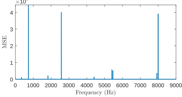
4.2.1 Fingerprint results

A scalar value damage indicator is dened, so it can now be applied over the full frequency range. The result can be seen in Figure 20, MSE from equation 13 is displayed on they-axis. The graph shows a few very high spikes (107_{) which make it an inconsistent and unreadable graph.}

0 1000 2000 3000 4000 5000 6000 7000 8000 9000

Frequency (Hz)

0 1 2 3 4

M

S

E

[image:29.595.146.446.205.365.2]

×107

Figure 20: Mean Square Error for all frequencies

The reason for these spikes is investigated. The rst local maximum, at 731 Hz, in Figure 20 is selected and the spectrum is viewed in Figure 21a. The middle amplitude is very low in relation to the rst sideband for the pristine case. This is also true for the damaged case, however considering the log scaley-axis, the dierence between these two cases is around a factor of 100. The impact that this has on the MSE is more easily identied by looking at the resulting ngerprint in Figure 21b. It can be concluded that this large dierence in the middle amplitude, which is used for normalisation, results in unusually large Mean Square Errors. Since this behaviour does not occur consistently and in varying levels throughout the frequency range, the method is deemed unstable.

710 715 720 725 730 735 740 745 750 Frequency (Hz)

10-10 10-8 10-6 10-4

A

m

p

li

tu

d

e

Pristine D50T

(a) FFT

1 2 3 4 5 6 7 8 9 10 11 12 13 14 15 16

Sideband Number

10-4 10-2 100 102 104 106

A

m

p

li

tu

d

e

Pristine D50T

(b) Fingerprint

Figure 21: Problem case Mean square error

4.2.2 Polynomial method results

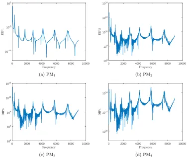
In the polynomial method, multiple possible indicators are mentioned to calculate the reaction to the damage. The main dierence with the ngerprint analysis is that here, the sideband amplitudes are not normalised. This makes the magnitude of the resulting damage indicator heavily dependent on the frequency, at the resonance the magnitude will be higher. All approaches have similar results in terms of shape, all need to be plotted on a log scale for comparison.

[image:29.595.104.479.515.667.2]

(30)

0 2000 4000 6000 8000 10000 Frequency

10-10 10-5 100

D

IP

1

(a) PM1

0 2000 4000 6000 8000 10000

Frequency

106 108 1010 1012 1014

D

IP

2

(b) PM2

0 2000 4000 6000 8000 10000

Frequency

104 106 108 1010 1012

D

IP

3

(c) PM3

0 2000 4000 6000 8000 10000

Frequency

1010 1012 1014

D

IP

4

[image:30.595.105.482.118.436.2]

(d) PM4

Figure 22: Polynomial method results from equations 15, 16, 17 & 18

One large dierence between the four is the magnitude itself, ranging from10−10_{in Figure 22a} to 1014 _{in Figure 22d. As is clear from the logarithmic} _{y-scale, the method is very volatile, the} magnitude of the damage indicator shifts too much over the frequency range for it to be a robust damage indicator.

4.2.3 RASTAR method results

In this method, all the sidebands in the spectrum are used to normalise the relative sideband amplitude to a percentage of the summation. As explained above, the amount of sidebands that are included in the calculation can be varied at will. The eect of changing the amount of included sidebands can be seen in Figure 23, all three are the pristine case compared to the D50T damage case. This method seems to behave more consistently. The indicator shows peak values at the anti-resonances. As expected, the lower frequencies show little change from using more sidebands, since the higher order terms do not hold much meaning for these frequencies. However, even for the higher frequencies, the lower amount of sidebands taken into account seem to result in a more sensitive indicator at the anti-resonances, but less at all other frequencies.

(31)

0 1000 2000 3000 4000 5000 6000 7000 8000 9000

Frequency (Hz)

0 10 20 30 40 50

S

u

m

ed

D

iff

er

en

ce

[image:31.595.154.440.120.251.2]

4 SBs 8 SBs 12 SBs

Figure 23: RASTAR method for 4,8 & 12 sidebands

The method yields fairly consistent values over the frequency range. Figure 23 shows the 50% damage case, which is a relatively excessive damage. To check the sensitivity the lower damage severities are also plotted in Figure 24. The indicator behaves as expected, a gradual increase in damage results in a gradual increase in damage indicator. The overall shape remains similar.

0 1000 2000 3000 4000 5000 6000 7000 8000 9000

Frequency (Hz)

0 5 10 15

S

u

m

ed

D

i

ff

er

en

ce

D10T D25T D50T

Figure 24: RASTAR method for three damage severities

The damage indicator should only indicate damage if there is any. Therefore, the pristine simulation is ran once more, this time with the excitation force halved. This should not change the dynamic behaviour of the sidebands, but only cause a vertical shift in overall amplitude. This case is then compared to the original pristine case and the D10T damage case, the smallest damage case. The result is shown in Figure 25. As can be seen, the blue line, which represents the damage indicator for the pristine case compared to the pristine case at low force, is non-existent in relation to the damaged case. The method works regardless of the input force. So this shows that just a vertical shift in the spectrum does not result in an indication for damage.

[image:31.595.156.440.360.490.2]