University of Warwick institutional repository: http://go.warwick.ac.uk/wrap
This paper is made available online in accordance with
publisher policies. Please scroll down to view the document
itself. Please refer to the repository record for this item and our
policy information available from the repository home page for
further information.
To see the final version of this paper please visit the publisher’s website.
Access to the published version may require a subscription.
Author(s): E.M. Watson, M.J. Chappell, F. Ducrozet, S.M. Poucher,
J.W.T. Yates
Article Title: A new general glucose homeostatic model using a
proportional-integral-derivative controller
Year of publication: 2011
Link to published article:
A New General Glucose Homeostatic Model using a
Proportional-Integral-Derivative Controller
E.M. Watsona,b,∗, M.J. Chappellb, F. Ducrozeta, S.M. Pouchera, J.W.T. Yatesa
aAstraZeneca, Discovery Department, Mereside, Alderley Park, Macclesfield, SK10 4TG,
UK
bUniversity of Warwick, School of Engineering, Gibbet Hill Road, Coventry, CV4 7AL, UK
Abstract
The glucose-insulin system is a challenging process to model due to the feedback mechanisms present, hence the implementation of a model-based approach to the system is an on-going and challenging research area. A new approach is proposed here which provides an effective way of characterising glycaemic regu-lation. The resulting model is built on the premise that there are three phases of insulin secretion, similar to those seen in a proportional-integral-derivative (PID) type controller used in engineering control problems. The model relates these three phases to a biological understanding of the system, as well as the logical premise that the homeostatic mechanisms will maintain very tight con-trol of the system. It includes states for insulin, glucose, insulin action and a state to simulate an integral function of glucose.
Structural identifiability analysis was performed on the model to determine whether a unique set of parameter values could be identidied from the available observations, which should permit meaningful conclusions to be drawn from pa-rameter estimation. Although two papa-rameters - glucose production rate and the proportional control coefficient - were found to be unidentifiable, the former is not a concern as this is known to be impossible to measure without a tracer
ex-∗Principle corresponding author ∗∗Corresponding author
Email addresses: E.M.Watson@warwick.ac.uk(E.M. Watson),
periment, and the latter can be easily estimated from other means. Subsequent parameter estimation using Intravenous Glucose Tolerance Test (IVGTT) and hyperglycaemic clamp data was performed and subsequent model simulations have shown good agreement with respect to these real data.
1. Introduction
Over recent decades much research has been devoted to the development of models that characterise the interaction between glucose and insulin. Probably the most widely known, accepted and applied model in this field is the Minimal Model (and its variants) introduced by Bergman et al. [1]. Previously, mod-els had been large and very complex in structure, whereas the Minimal Model is, as the name suggests, minimal in terms of its structure and the number of key system parameters that it includes. In particular, the Minimal Model also includes in its structure a very important parameter representing insulin sensitivity, which is a measure of how much glucose is removed from the blood per unit of insulin. In certain situations the Minimal Model is a very useful tool, however in others it does not necessarily meet expectations as shown by De Gaetano et al.[2]. For example, insulin secretion with the minimal model is stopped after the glucose level falls below a certain threshold, making it invalid once the system has returned to a steady state.
More recently, a Beta Cell Mass Model has been developed by Topp et al.[3]. Unlike the Minimal Model, it is concerned with a long-term view of glucose-insulin dynamics and includes an additional compartment to represent β-cell mass. While this model appears to predict long-term aspects of the system and disease progression well, it lacks a representation of insulin delay and insulin se-cretion is geared to a steady state, which makes it far less useful for short-term modelling.
Jauslin/Silber[4] have also developed an alternative model to characterise glucose-insulin interaction. The Jauslin/Silber model follows standard pharmacokinetic structures and attempts to be applicable to both Oral Glucose Tolerance Tests (OGTTs) and Intravenous Glucose Tolerance Tests (IVGTTs) in both healthy and type 2 diabetic patients. Using this model and the data collected to look at 24 hour profiles of these subjects, aspects of the insulin effect compartment have been incorporated into the design of the model presented here.
both animals and man. If the glucose level is elevated above normal (hypergly-caemia), its toxic effect can damage blood vessels, nerves and other important body systems. When the blood glucose level is raised, the endothelial cells that line the blood vessels absorb more glucose than normal, leading the blood vessels to grow thicker and weaker which reduces blood flow throughout the body. This can cause retinopathy leading to vision loss, neuropathy (loss of sensation) and, in severe cases, amputation is necessary. Other potential complications include nephropathy, which may require dialysis or kidney transplant, heart attacks, strokes and muscle wasting. If the glucose level falls too low (hypoglycaemia), there is insufficient energy to sustain normal function of the central nervous sys-tem, which may result in coma and even death. For a full review of the eitology of type 2 diabetes see Haffner [5].
To prevent serious damage such as that detailed above, the glucose-insulin home-ostatic system is crucial and is therefore normally very finely controlled. It is critically damped or even very slightly over-damped, keeping it close to a steady state or a fixed point with little overshoot and returning high levels of glucose rapidly back to the fixed point show by Bolie[6].
2. The Model
2.1. Modelling Approach
The aim of the modelling approach undertaken here was to create a unified, robust model for the glucose-insulin system that would:
• Be applicable to a variety of different clinical tests, such as an IVGTT and hyperglycaemic or euglycaemic clamps.
• Be stable, robust (e.g. not having an output which increases exponentially over time) and ensure that meaningful results would be produced even with large variations between subjects.
dia-betes or in an animal model such as a Zucker rat model shown in [7]. Another example would be high fasted glucose levels where a subject has uncontrolled type 2 diabetes.
It is desirable to have a model that is minimal in form, but it must still contain sufficient structural parameters to accurately model the physical system. It must therefore contain only necessary components and have only one set of parameters per individual, but provide enough flexibility to explain variation between subjects. In order to ensure that the model remains valid in extreme situations, it should adhere to biological theory in such a way that parameter difference between subjects represents different physical attributes. The model should use familiar concepts so it is easily understood and can be applied by both the mathematical/engineering community and the pre-clinical and clinical bioscience community.
2.2. Model Concept
Various engineering disciplines require a very fine level of control to be main-tained over systems - chemical synthesis processes, for example, may require fine control over water temperature. Control could be achieved using a thermostat, where a heater is switched on or off depending on the water temperature, how-ever this would not give sufficiently accurate control for some situations, such as distilling in [8], so engineers have developed more accurate controllers specif-ically for this task. The human body requires similar levels of fine control for its homeostatic mechanisms. It is a logical conclusion that both human design and the process of evolution may have developed an appropriate solution in the form of a similar controller.
proportional, which is a multiple of the error signal, integral, the area under the curve of the error signal, and differential, the rate of change of the error signal. A PID controller has also been used as a method of controlling glucose levels in type 1 diabetics, i.e. those diabetics who do not secrete any insulin. There have been attempts to produce an artifical pancreas using continous glucose monitors with a PID controller to regulate the infusion of insulin[10, 11, 12, 13, 14, 15]. To the authors’ knowledge, there has been no attempt to use a PID controller as an analogy for β-cells in an attempt to explain how they function. The controller can be shown to fit with the way that the beta cells in the pancreas secrete insulin:
Proportional:
• In mathematical terms, this means that for every unit of plasma glucose, a fixed amount of insulin is released by the pancreas. See Figure 3.
• This part of the controller simulates the secretion in basal conditions. The proportional aspect maintains a basal level of glucose in the system and a basal level of insulin to match.
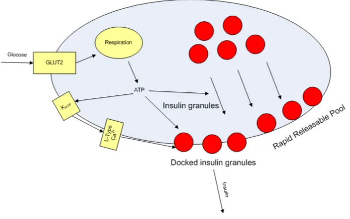
• In biological terms, this means that glucose enters the beta cell which, via glycolysis and oxidative phosphorylation, increases the level of ATP [16]. In the proportional controller analogy, the ATP predominantly promotes granules of pro-insulin towards the membrane. See Figure 1.
Integral:
• In mathematical terms, this is the area under the curve (AUC) of the glucose concentration.
• This part simulates the second phase insulin response: the shoulder of insulin observed after an IVGTT.
This represents the amount of insulin required to remove the glucose after a meal, sugar intake or clinical challenge.
Derivative:
• In mathematical terms, this is the rate of change of glucose level.
• This part represents the first phase insulin response: the relatively high amount of insulin that is seen initially in experiments such as IVGTT.
• In biological terms, this could mean that the docked insulin granules on the cell membrane are predominantly released in a rapid response to a large increase in the amount of glucose present. It gives a measured response to sudden, large changes in concentration of glucose but has little effect when levels rise slowly.
<<Figure 1 in here >>
The model presented here is split into three sections: Insulin Secretion (I(t)
andIi(t)), Delayed Insulin Action (Ia(t)), and Net Difference in GlucoseG(t)).
2.3. Insulin Secretion
The basal levels of glucose and insulin are not fixed points in the biological mechanism. Instead, they are determined by the effect they have on each other in their steady states. The Beta Cell Mass Model [3] has been developed in this way; the basal levels of each are not defined, but are determined by the combi-nation of parameters used. The model shows what can happen in the system if a reduction of insulin sensitivity occurs.
this is not quite a valid analogy as a biological system does not have a defined set point, so the challenge is to design a model with similar terms to those present in a PID Controller without a set point.
The terms in the PID controller relate to the biological process as follows: Proportional: kpG(t)
This term simply creates the basal level under static conditions. The pro-portional secretion rate is produced by taking the level present in the glucose compartment.
Integral: kiIi(t)
This is non-trivial as the area under the glucose curve will increase over time, causing the system to become unstable. Hence the integral function must decay over time when the system tends towards steady state. It is created by taking the concentration in the glucose compartment as the rate of change of a virtual compartmentIi(t).
dIi(t)
dt =G(t)−kiirIi(t) (1)
Derivative: kd dG(t)
dx
This is a rate of change, so the absolute value of the glucose does not matter. This is simply taken as the rate of change of glucose, and is incorporated in the following equation:
dI(t)
dt =kpG(t) +kiIi(t) +kd dG(t)
dt −iirI(t) (2) 2.4. Delayed Insulin Action
In the tests shown below, the IVGTT and the hyperglycaemic clamp both start with an elevated level of glucose. As insulin and glucose are both drivers of glucose disposal rate, as illustrated by equation 4, it is difficult to distinguish whether the high glucose disposal rate is due to the elevated glucose level, the corresponding elevated insulin level or both. Therefore, from the tests below, it is difficult to establish whether a delay in insulin action is present; however, based on evidence from the literature that a delay should be present, it has been decided that a delay should be incorporated into the model.
In order to include this delay in the model, an insulin action compartment,
Ia(t), was incorporated. This compartment is the same as the interstitial
com-partment in the Minimal Model, but is rearranged here for easy interpretation ofthe parameters:
dIa
dt =I(t)−kiarIa(t) (3)
wherekiar is the clearance rate from the insulin action compartment.
2.5. Net Difference in Glucose
The glucose compartment has a number of inputs (which are impossible to determine without tracer experiments, [21]) and a number of outputs. The relative rates of supply and dispersal of glucose in this compartment determine the basal level. This is modelled in a clear manner in the Beta Cell Mass Model [3]; it has an appearance rate that is made up of all unknown appearance rates and all the disposal rates that can be calculated. The appearance rate cannot be established without tracer experiments, however as appearance rate is related to the amount of glucose present, obtaining an absolute value is unimportant. Insulin has an effect on both the production rate of glucose and its disposal rate, however it is impossible to distinguish and quantify the effect on each as the end result is the same.
This provides us with three key parameters (shown in equation (4)):
• Glucose Effectiveness, which describes the insulin-independent removal of glucose (i.e. the removal of glucose based on glucose concentration alone),
gr.
• Insulin Sensitivity, which is the net effect of insulin on lowering the glucose level,ksi.
dG(t)
dt =gp−(gr+ksi.Ia(t)).G(t) (4)
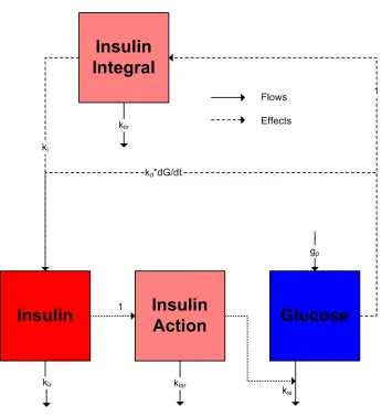
Figure (2) summarises the model.
<< Figure 2 in here>>
<<Figure 3 in here >>
3. Steady States
As mentioned above, unlike some previous models this system does not have steady states dependent on parameters such as glucose and insulin basal levels. The system should tend to steady states based on the system parameters and the feedback components present.
At steady state, nothing is changing hence the derivative term in the model is zero. With a classic PID controller, there is an error signal entering the con-troller; however this is not the case with this system as there is no “set point” to derive an error signal from. The integral control is therefore required to in-troduce decay. This makes the calculations slightly complex as the steady state for this parameter is non-zero.
From the system equations (1)-(4) the steady states can be calculated alge-braically, for example from equation (1) we have:
Iiss= Gss kiir
(5)
Adding in the proportional control, the steady state for insulin becomes:
Iss=
kiIiss+kpGss kir
From equation 3 the steady state for insulin action is given by:
Iass= Iss kiar
(7) and the resulting steady state for glucose is given by:
Gss =
gp gr+ksi·Iass
(8)
These can be calculated from the system equations algebraically.
4. Structural Identifiability
The problem with using a simplistic model, such as a 2-compartment model, is that it does not capture all the dynamics of the system - such as the variable insulin dynamics created by rapid changes in glucose [22] - and hence is not an accurate representation. On the other hand, a pathway model would require a larger number of parameters which would allow different combinations of val-ues to produce the same system output. As a variety of different parameter combinations could be used to fit the same data, it would be impossible to tell which was actually correct; this would make it impossible to validate the model and therefore render it practically useless. The solution is to create a model which is a balance between these two approaches, by using not only parameters that can be uniquely identified but also a mechanistic structure that adequately describes the physical process and dynamics that are observed. This creates a need for a test to validate the model by ensuring that all parameters can be uniquely identified.
is just a representation of an integral function. The model was treated as an uncontrolled non-linear system. All the parameters including initial conditions were considered unknown. There are various techniques for performing a struc-tural identifiability analysis, [23]. The Lie-symmetry approach by Yates et al. [24] has been applied to the model introduced here, as other techniques such as the Taylor series approach could not yield a solution due to computational difficulties. The analysis is presented in the appendix and was performed using Mathematica 7 [25]. Mathematica was selected for the analysis as it is excellent for complex symbolic manipulation and performing the analysis by hand would be time-consuming and error-prone. System Observability is a prerequisite for the Lie-symmetry technique, so the Observability Rank Criterion was applied to the model with observations ofG(t) andI(t), which showed it to be observable. Application of this approach concluded that the model is at least locally iden-tifiable (as global identifiability cannot be established with the Lie-symmetry approach) when two parameters were known: gp, which represents glucose
pro-duction, andkp, the proportional insulin secretion function; other insulin
secre-tion terms could be used instead, however it is easier to consider the proporsecre-tional control as it can be calculated at basal states.
This leads to issues with the following parameters:
gp - This represents the amount of glucose entering the system, which is
typ-ically unknown. It can be set to an estimate, perhaps obtained from a tracer experiment, as the clearance is fractional so an exact value is not necessary.
kp - The proportional insulin secretion function is more difficult to estimate,
however assuming that that the integral component is negligible at steady state a rough estimate forkp can be obtained using the known insulin clearance with
this expression which has been derived from the steady state.
kp≈
irIbasal Gbasal
5. Parameter Estimation
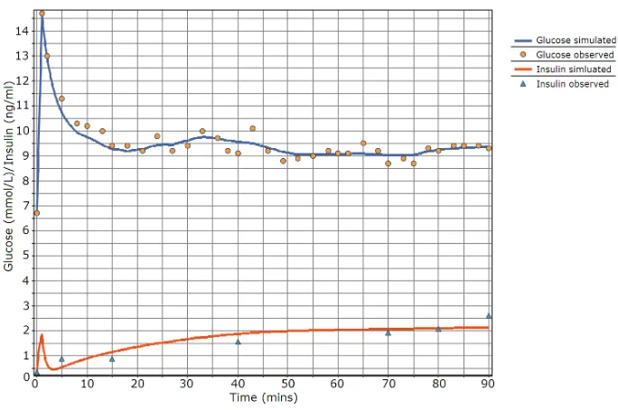
The data used for parameter estimation were rat data (IVGTT and hy-perglycaemic clamps) from AstraZeneca and data obtained from an IVGTT experiment on a healthy human and previously used with the Minimal Model and the program MINMOD by [26]. The data were fitted using acslX 2.5 [27] and a PKPD toolkit developed at AstraZeneca. Fitting was performed using a Quasi-Newton optimisation algorithm and the built-in Gear’s Stiff Integration algorithm. This was performed on a standard PC (Windows XP SP3, 2GB RAM, 1.66 GHz Intel Core 2 Duo) within a few seconds. See Figures 4-6 and Table 2 for the fitted parameters. The description of the parameters is in Table 1. The parameter fitting and subsequent model simulation provide good agree-ment compared to experiagree-mental data, and similar parameter values can be used across animals (noting that the animals in the clamp and the IVGTT are dif-ferent hence the slight difference in values). An important point to note is that
kd is not well-fitted with respect to the hyperglycaemic clamp experiment due
to the lack of data at the start of the clamp. All other parameters estimates are within 20% of their correct value with 95% confidence. The parameter values have been adjusted slightly as without all the components of the controller, the model does not control the glucose levels in the simulation.
<< Table 1 in here>>
<< Table 2 in here>>
<< Figure 4 in here>>
<< Figure 5 in here>>
<< Figure 6 in here>>
6. Discussion
(kp,ki,kd,kir) derived from the PID controller type terms incorporated in the
model structure for glucose-stimulated insulin secretion (GSIS) and may help to identify and differentiate between the effect of drugs or incretins such as GIP and GLP-1 by showing an increase in one or more of the PID parameters. This allows clearer observation of external influences (such as drugs or disease) af-fecting mechanisms in the pancreas. It can also help identify which part of the glucose-insulin homeostasis is impaired, providing a better understanding of the mechanism of insulin resistance in type 2 diabetics.
The insulin sensitivity (ksi) and glucose removal rate (gr) are clearly defined,
making it easy to identify the difference between subjects.
This paper introduces a new concept for the glucose-insulin model, in particular the PID approach to insulin secretion terms. Other models have included insulin secretion terms; for example the Minimal Model [1], although this does not have a first-phase insulin secretion term, and the DIST and DISTq models [28, 29], though these use larger numbers of parameters than the model presented here. Insulin sensitivity in this model was based on the interstitial insulin compart-ment from the Minimal Model, however there are valid alternative methods to calculate insulin sensivity[30].
other models may fail. For instance, if the first phase of insulin secretion was decreased, this would be reflected in the derivative parameter (kd). These are
all factors that are to be included in future work and development of the model. Models and control systems for managing glucose homeostatics are becoming increasingly important with current developments in constant glucose moni-toring ([33]) in conjunction with the use of insulin pumps. A PID controller has been used to attempt to manage glucose with an artifical pancreas by [10, 11, 12, 13, 14, 15], an approach which seems to be supported by this work. It is interesting to note that when a PID controller has been used in an artifical pancreas in practice it caused glucose levels to drop too low, which meant that another attempt was made using just a PI controller (i.e. one with no differential term) however the differential term was determined well in the paper [34].
7. Acknowledgments
Thanks goes to Alice Yu and Ruth MacDonald from AstraZeneca for per-forming the rat IVGTT and hyperglycaemic clamp, which where carried out under the Animal (Scientific Procedures) Act 1986. Thanks also goes to As-traZeneca for funding this research.
References
[1] R. Bergman, Y. Ider, C. Bowden, C. Cobelli, Quantitative estimation of insulin sensitivity, Am.J.Physiol. 236 (6) (1979) E667–E677.
[2] A. De Gaetano, O. Arino, Mathematical modelling of the intravenous glu-cose tolerance test, J.Math.Biol. 40 (2) (2000) 136–168.
[4] H. E. Silber, P. M. Jauslin, N. Frey, R. Gieschke, U. S. Simonsson, M. O. Karlsson, An integrated model for glucose and insulin regulation in healthy volunteers and type 2 diabetic patients following intravenous glucose provo-cations, J Clin Pharmacol 47 (9) (2007) 1159–1171.
[5] S. Haffner, Type 2 diabetes: Unravelling its causes and consequences: A compendium of classical papers, Cambridge: Medical Publications, (2002).
[6] V. W. Bolie, Coefficients of normal blood glucose regulation, J.Appl.Physiol. 16 (5) (1961) 783–788.
[7] B. Kasiske, M. O’Donnell, W. Keane, The zucker rat model of obesity, insulin resistance, hyperlipidemia, and renal injury, Hypertension 19 (1 Suppl) (1992) I110–I115.
[8] M. Vester, R. Van der Linden, J. Pangels, Control design for an industrial distillation column, Computers & Chemical Engineering 17 (5-6) (1993) 609–615.
[9] C. Bissell, Control Engineering, Vol. 2nd Revised edition, CRC Press, (1994).
[10] G. M. Steil, A. E. Panteleon, K. Rebrin, Closed-loop insulin delivery-the path to physiological glucose control, Adv Drug Deliv Rev 56 (2004) 125– 44.
[11] G. M. Steil, B. Clark, S. Kanderian, K. Rebrin, Modeling insulin action for development of a closed-loop artificial pancreas, Diabetes Technol Ther 7 (2005) 94–108.
[12] C. V. Doran, N. H. Hudson, K. T. Moorhead, J. G. Chase, G. M. Shaw, C. E. Hann, Derivative weighted active insulin control modelling and clin-ical trials for ICU patients, Med Eng Phys 26 (2005) 94–108.
[14] K. A. Wintergerst, D. Deiss, B. Buckingham, M. Cantwell, S. Kache, S. Agarwal, D. M. Wilson, G. Steil, Glucose control in pediatric inten-sive care unit pateints using an insulin-glucose algorithm, Diabetes Technol Ther 9 (2008) 211–22.
[15] G. Steil, K. Rebrin, J. J. Mastrototaro, Metabolic modelling and the closed-loop insulin delivery problem, Diabetes Research and Clinical Practice 74 (Supplement 2) (2006) S183–S186.
[16] D. Langin, Diabetes, insulin secretion, and the pancreatic beta-cell mito-chondrion, N.Engl.J.Med. 345 (24) (2001) 1772–1774.
[17] T. Bratanova-Tochkova, H. Cheng, S. Daniel, S. Gunawardana, Y. Liu, J. Mulvaney-Musa, T. Schermerhorn, S. Straub, H. Yajima, G. Sharp, Trig-gering and augmentation mechanisms, granule pools, and biphasic insulin secretion, Diabetes 51 Suppl 1 (2002) S83–S90.
[18] E. R. Carson, C. Cobelli, Modelling methodology for physiology and medicine, San Diego, Calif. ; Academic, c2001.
[19] A. Natali, A. Gastaldelli, S. Camastra, A. M. Sironi, E. Toschi, A. Masoni, E. Ferrannini, A. Mari, Dose-response characteristics of insulin action on glucose metabolism: a non-steady-state approach, Am J Physiol Endocrinol Metab 278 (2000) 794–801.
[20] R. L. Prigeon, M. E. Roder, J. Porte, D., S. E. Kahn, The effect of insulin dose on the measurement of insulin sensitivity by the minimal model tech-nique. Evidence for saturable insulin transport in humans, J Clin Invest 97 (1996) 501–7.
[22] J. J. Lima, N. Matsushima, N. Kissoon, J. Wang, J. E. Sylvester, W. J. Jusko, Modeling the metabolic effects of terbutaline in [beta]2-adrenergic receptor diplotypes[ast], Clin Pharmacol Ther 76 (1) (2004) 27–37.
[23] M. J. Chappell, K. Godfrey, S. Vajda, Global identifiability of the param-eters of nonlinear systems with specified inputs: a comparison of methods, Math.Biosci. 102 (1) (1990) 41–73.
[24] J. W. Yates, N. D. Evans, M. J. Chappell, Structural identifiability analysis via symmetries of differential equations, Automatica 45 (11) (2009) 2585 – 2591. doi:DOI: 10.1016/j.automatica.2009.07.009.
[25] Wolfram, Mathematica (2009).
URLhttp://www.wolfram.com/
[26] G. Pacini, R. Bergman, Minmod: a computer program to calculate insulin sensitivity and pancreatic responsivity from the frequently sampled intra-venous glucose tolerance test, Comput.Methods.Programs.Biomed. 23 (2) (1986) 113–122.
[27] AEgis, acslx (2008).
URLhttp://www.acslx.com/
[28] P. Docherty, J. Chase, T. Lotz, C. Hann, G. Shaw, J. Berkeley, J. Mann, K. McAuley, DISTq: An iterative analysis of glucose data for low-cost, real-time and accurate estimation of insulin sensitivity, The Open Medical Informatics Journal 3 (2009) 65–76.
[29] T. F. Lotz, J. G. Chase, K. A. McAuley, G. M. Shaw, X. W. Wong, J. Lin, A. Lecompte, C. E. Hann, J. I. Mann, Monte Carlo analysis of a new model-based method for insulin sensitivity testing, Comput Method Programs Biomed 89 (2008) 215–25.
[31] R. Watanabe, R. Bergman, Accurate measurement of endogenous insulin secretion does not require separate assessment of c-peptide kinetics, Dia-betes 49 (3) (2000) 373–382.
[32] M. O’Connor, H. Landahl, G. Grodsky, Comparison of storage- and signal-limited models of pancreatic insulin secretion, Am.J.Physiol. 238 (5) (1980) R378–R389.
[33] F. R. Kaufman, L. C. Gibson, M. Halvorson, S. Carpenter, L. K. Fisher, P. Pitukcheewanont, A pilot study of the continuous glucose monitoring system: Clinical decisions and glycemic control after its use in pediatric type 1 diabetic subjects, Diabetes care 24 (12) (2001) 2030–2034.
Appendix:Mathematica Code
Load the Lie group package in to Mathematica. (The output from the package is suppressed)
Needs["SymmetryAnalysis`IntroToSymmetry`"]; Needs["SymmetryAnalysis`IntroToSymmetry`"]; Needs["SymmetryAnalysis`IntroToSymmetry`"]; Defines the differential equations:
inputequation1="D[x1[t],t]-p[4]+ (p5[t] +(p6[t] *x4[t]))*x1[t]"; inputequation1="D[x1[t],t]-p[4]+ (p5[t] +(p6[t] *x4[t]))*x1[t]"; inputequation1="D[x1[t],t]-p[4]+ (p5[t] +(p6[t] *x4[t]))*x1[t]";
inputequation2="D[x2[t],t] -p[7]*x1[t] +p10[t]*x2[t] - x3[t]*p8[t]- p9[t]*D[x1[t],t]"; inputequation2="D[x2[t],t] -p[7]*x1[t] +p10[t]*x2[t] - x3[t]*p8[t]- p9[t]*D[x1[t],t]"; inputequation2="D[x2[t],t] -p[7]*x1[t] +p10[t]*x2[t] - x3[t]*p8[t]- p9[t]*D[x1[t],t]"; inputequation3="D[x3[t],t]-x1[t]+ p11[t]*x3[t]";
inputequation3="D[x3[t],t]-x1[t]+ p11[t]*x3[t]"; inputequation3="D[x3[t],t]-x1[t]+ p11[t]*x3[t]"; inputequation4="D[x4[t],t]-x2[t]+p12[t]*x4[t]"; inputequation4="D[x4[t],t]-x2[t]+p12[t]*x4[t]"; inputequation4="D[x4[t],t]-x2[t]+p12[t]*x4[t]"; inputequation5="D[p4[t],t]";
inputequation5="D[p4[t],t]"; inputequation5="D[p4[t],t]"; inputequation6="D[p5[t],t]"; inputequation6="D[p5[t],t]"; inputequation6="D[p5[t],t]"; inputequation7="D[p6[t],t]"; inputequation7="D[p6[t],t]"; inputequation7="D[p6[t],t]"; inputequation8="D[p7[t],t]"; inputequation8="D[p7[t],t]"; inputequation8="D[p7[t],t]"; inputequation9="D[p8[t],t]"; inputequation9="D[p8[t],t]"; inputequation9="D[p8[t],t]"; inputequation10="D[p9[t],t]"; inputequation10="D[p9[t],t]"; inputequation10="D[p9[t],t]"; inputequation11="D[p10[t],t]"; inputequation11="D[p10[t],t]"; inputequation11="D[p10[t],t]"; inputequation12="D[p11[t],t]"; inputequation12="D[p11[t],t]"; inputequation12="D[p11[t],t]"; inputequation13="D[p12[t],t]"; inputequation13="D[p12[t],t]"; inputequation13="D[p12[t],t]";
Associated substitution rules are also defined to aid the symmetry package: rulesarray={"D[x1[t],t]->-(-p4[t]+ (p5[t] +(p6[t] *x4[t]))*x1[t])",
rulesarray={"D[x1[t],t]->-(-p4[t]+ (p5[t] +(p6[t] *x4[t]))*x1[t])", rulesarray={"D[x1[t],t]->-(-p4[t]+ (p5[t] +(p6[t] *x4[t]))*x1[t])",
"D[x2[t],t] ->-(-p7[t]*x1[t] +p10[t]*x2[t] - x3[t]*p8[t]- p9[t]*x1[t])",
"D[x2[t],t] ->-(-p7[t]*x1[t] +p10[t]*x2[t] - x3[t]*p8[t]- p9[t]*x1[t])",
"D[x2[t],t] ->-(-p7[t]*x1[t] +p10[t]*x2[t] - x3[t]*p8[t]- p9[t]*x1[t])",
"D[x3[t],t]->-(-x1[t]+ p11[t]*x3[t])",
"D[x3[t],t]->-(-x1[t]+ p11[t]*x3[t])",
"D[x3[t],t]->-(-x1[t]+ p11[t]*x3[t])",
"D[x4[t],t]->x2[t]-p12[t]*x4[t]","D[p4[t],t]->0",
"D[x4[t],t]->x2[t]-p12[t]*x4[t]","D[p4[t],t]->0",
"D[x4[t],t]->x2[t]-p12[t]*x4[t]","D[p4[t],t]->0",
"D[p5[t],t]->0",
"D[p5[t],t]->0",
"D[p5[t],t]->0",
"D[p6[t],t]->0",
"D[p6[t],t]->0",
"D[p6[t],t]->0",
"D[p7[t],t]->0",
"D[p7[t],t]->0",
"D[p7[t],t]->0",
"D[p8[t],t]->0",
"D[p8[t],t]->0",
"D[p8[t],t]->0",
"D[p9[t],t]->0",
"D[p9[t],t]->0",
"D[p9[t],t]->0",
"D[p10[t],t]->0",
"D[p10[t],t]->0",
"D[p10[t],t]->0",
"D[p11[t],t]->0",
"D[p11[t],t]->0",
"D[p12[t],t]->0"};
"D[p12[t],t]->0"};
"D[p12[t],t]->0"};
Independent and dependent variables are defined: independentvariables={"t"};
independentvariables={"t"}; independentvariables={"t"};
dependentvariables={"x1","x2","x3","x4","p4","p5","p6", dependentvariables={"x1","x2","x3","x4","p4","p5","p6", dependentvariables={"x1","x2","x3","x4","p4","p5","p6",
"p7","p8","p9","p10","p11","p12"};
"p7","p8","p9","p10","p11","p12"};
"p7","p8","p9","p10","p11","p12"};
Package parameters are defined: frozennames ={""};
frozennames =frozennames ={{""""}};;
p= 1;
pp= 1;= 1;
r= 0;
rr= 0;= 0; xseon = 1; xseon = 1;xseon = 1; internalrules = 1; internalrules = 1;internalrules = 1;
The Lie symmetries are derived for the differential equations:
FindDeterminingEquations[independentvariables,dependentvariables,frozennames,
FindDeterminingEquations[independentvariablesFindDeterminingEquations[independentvariables,,dependentvariablesdependentvariables,,frozennamesfrozennames,, p, r,xseon,inputequation1,rulesarray,internalrules];
p, r,p, r,xseonxseon,,inputequation1inputequation1,,rulesarrayrulesarray,,internalrules];internalrules]; zdeterminingequations1 = zdeterminingequations; zdeterminingequations1 = zdeterminingequations;zdeterminingequations1 = zdeterminingequations; Repeated for ever inputequationinputequationinputequation and then joined:
zdeterminingequations = Join[zdeterminingequations1,zdeterminingequations2,
zdeterminingequations = Join[zdeterminingequations1zdeterminingequations = Join[zdeterminingequations1,,zdeterminingequations2zdeterminingequations2,,
zdeterminingequations3,zdeterminingequations4,zdeterminingequations5,
zdeterminingequations3zdeterminingequations3,,zdeterminingequations4zdeterminingequations4,,zdeterminingequations5zdeterminingequations5,,
zdeterminingequations6,zdeterminingequations7,zdeterminingequations8,
zdeterminingequations6zdeterminingequations6,,zdeterminingequations7zdeterminingequations7,,zdeterminingequations8zdeterminingequations8,,
zdeterminingequations9,zdeterminingequations10,zdeterminingequations11,
zdeterminingequations9zdeterminingequations9,,zdeterminingequations10zdeterminingequations10,,zdeterminingequations11zdeterminingequations11,,
zdeterminingequations12,zdeterminingequations13]; zdeterminingequations12zdeterminingequations12,,zdeterminingequations13];zdeterminingequations13];
The determining equations are solved up to symmetries of polynomial order 1: SolveDeterminingEquations[independentvariables,dependentvariables,r, SolveDeterminingEquations[independentvariables,dependentvariables,r, SolveDeterminingEquations[independentvariables,dependentvariables,r, xseon,zdeterminingequations,1] xseon,zdeterminingequations,1] xseon,zdeterminingequations,1]
The symmetries of the differentual equations are displayed: TableForm[xsefunctions]
TableForm[xsefunctions] TableForm[xsefunctions]
xse1=a10 + a12*z10 + a13*z11 + a14*z12 + a15*z13 + a16*z14 + a111*z6 + a112*z7 + a113*z8 + a114*z9 TableForm[etafunctions]
TableForm[etafunctions] TableForm[etafunctions] eta1=0
eta3=0 eta4=0
eta5=b50 + b52*z10 + b53*z11 + b54*z12 + b55*z13 + b56*z14 + b511*z6 + b512*z7 + b513*z8 + b514*z9 eta6=0
eta7=0
eta8=b80 + b82*z10 + b83*z11 + b84*z12 + b85*z13 + b86*z14 + b811*z6 + b812*z7 + b813*z8 + b814*z9 eta9=0
eta10=0 eta11=0 eta12=0 eta13=0
The conditions are that the perturbation on time, xse1, must be zero. Only eta5 and eta8 are non-zero which means they are unidentifiable. eta5 relates to p4 which isgp and eta8 relates to p7 which is kd. See structural identifiability
Figure Captions
Figure 1:Diagram of the beta-cell to show the elements of it that relate to the terms in the PID controller.
Figure 2:Schematic diagram of the PID model of the glucose and insulin system. Figure 3:The elements of the PID controller split up to show their individual influence on insulin secretion in the model.
Figure 4:Parameter fit of a human IVGTT using the PID model with data from [26].
Figure 5:Parameter fit of a rat IVGTT using the PID model.
Table Captions
Table 1: Description of the parameters in PID model.
Parameter Units Description
gr min−1
Glucose Effectiveness, insulin-independent glucose removal (most of the glucose removal in this test is determined by insulin hence the insensitivity)
gp mmol l−1min−1 Glucose production rate
ksi ml ng−1 Insulin sensitivity, insulin-dependent glucose removal kp µg mmol−1 min−1 Proportional parameter for PID model
ki µg mmol−1 min−2 Integral parameter for PID model kd µg mmol−1 Differential parameter for PID model kir min−1 Insulin clearance
kiir min−1 Integral clearance rate, to simulate integral function kiar min−1 Insulin action increase rate, to delay insulin action G0 mmol l−1 Starting glucose
I0 µg l−1 Starting insulin
[image:26.612.133.527.242.537.2]Ia0 mmol l−1min Starting insulin action (non-sensitive parameter) Ii0 µg l−1 min Starting insulin integral (non-sensitive parameter)
Parameter Human Han Wistar Han Wistar Units IVGTT IVGTT Hyperglycaemic Clamp
gr 0.00159 0.0438 0.0413 min−1
gp [3] 0.033 0.033 0.033 mmol l−1min−1
ksi 0.00231 0.00105 0.00107 ml ng−1
kp (Equation 9) 0.0275 0.009274 0.00896 µg mmol−1 min−1 ki 0.00000158 0.000872 0.000256 µg mmol−1 min−2
kd 0.268 0.450 0.455 µg mmol−1
kir 0.169 0.351 0.118 min−1
kiir 1.38E-19 1.38E-19 1.38E-19 min−1
kiar 0.114 0.0296 0.258 min−1
G0 5.11 5.8 6.7 mmol l−1
I0 0.379 0.879 0.348 µg l−1
Ia0 0 0 0 mmol l−1min
[image:27.612.134.543.253.530.2]Ii0 0 0 0 µg l−1 min
+ +
+
+
++ +
+ +
++ ++
+ + +
+ + + +
+ + + +
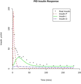
+ Real Insulin Insulin P Insulin I Insulin D
PID Insulin Response
Time (mins)
Insulin
µ
U/ml
0
50
100
150
[image:30.612.161.421.237.507.2]0 50 100 150 200
Figure 4: Parameter fit of a human IVGTT using the PID model with data from [26].
[image:31.612.134.464.419.635.2]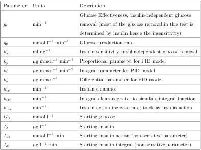
![Table 2: Fitted parameter estimates in the PID model using data from AstraZeneca and [26].](https://thumb-us.123doks.com/thumbv2/123dok_us/9671756.468999/27.612.134.543.253.530/table-fitted-parameter-estimates-pid-model-using-astrazeneca.webp)
![Figure 4: Parameter fit of a human IVGTT using the PID model with data from [26].](https://thumb-us.123doks.com/thumbv2/123dok_us/9671756.468999/31.612.134.464.419.635/figure-parameter-t-human-ivgtt-using-pid-model.webp)