A comparison of Markov functional and market models : the one dimensional case

University of Warwick institutional repository: http://go.warwick.ac.uk/wrap

This paper is made available online in accordance with publisher policies. Please scroll down to view the document itself. Please refer to the repository record for this item and our policy information available from the repository home page for further information.

To see the final version of this paper please visit the publisher’s website. Access to the published version may require a subscription.

Author(s): MN Bennett and JE Kennedy

Article Title: A Comparison of Markov-Functional and Market Models: The One-Dimensional Case

Year of publication: 2005 Link to published article:

http://dx.doi.org/10.3905/jod.2005.605351

Publisher statement: This is the submitted version of the following article: A Comparison of Markov-Functional and Market Models: The One-Dimensional Case, M. N. Bennett and J. E. Kennedy, The Journal of Derivatives, Vol. 13(2), © 2005, Institutional Investor, Inc., which has been published in final form at:

A Comparison of Markov-Functional and

Market Models: The One-Dimensional Case

Michael N. Bennett, Joanne E. Kennedy

University of Warwick

July 25, 2005

Abstract

The LIBOR Markov-functional model is an efficient arbitrage-free pricing model suitable for callable interest rate derivatives. We demonstrate that the dimensional LIBOR Markov-functional model and the separable one-factor LIBOR market model are very similar. Consequently, the intuition behind the familiar SDE formulation of the LIBOR market model may be applied to the LIBOR Markov-functional model.

The application of a drift approximation to a separable one-factor LIBOR market model results in an approximating model driven by a one-dimensional Markov process, permitting efficient implementation. For a given parameteri-sation of the driving process, we find the distributional structure of this model and the corresponding Markov-functional model are numerically virtually indistinguishable for short maturity tenor structures over a wide variety of market conditions, and both are very similar to the market model. A theoret-ical uniqueness result shows that any accurate approximation to a separable market model that reduces to a function of the driving process is effectively an approximation to the analogous Markov-functional model. Therefore, our conclusions are not restricted to our particular choice of driving process. Mi-nor differences are observed for longer maturities, nevertheless the models remain qualitatively similar. These differences do not have a large impact on Bermudan swaption prices.

1

Introduction

The problem of pricing callable exotic interest rate derivatives, such as the Bermudan swaption, is one of the most important problems in option pricing theory, being of great practical importance in the marketplace. The LIBOR market model of interest rate dynamics, developed by Brace, G¸atarek & Musiela [1997], Milterson, Sandmann & Sondermann [1997], and to a lesser extent the corresponding swap-based market model developed by Jamshidian [1997], have now become some of the most popular models for pricing such derivatives. They are generally considered to have more desirable theoretical calibration properties than short-rate models such as the Vasicek-Hull-White model (Hull & White [1990]). However, the high dimensionality of the full market model specification means that it is usually desirable to approximate the model in some way to obtain an efficient pricing algorithm.

show that under such a model the drift-approximated forward LIBORs may be written as a function of a one-dimensional Markov process of the form

xt :=

Z t

0

σs dWs. (1)

We will henceforth refer to this approximate pricing model as the drift

ap-proximation model. We shall see that the concept of separability introduced

in the construction of this efficient model provides the link between market models and Markov-functional models.

The LIBOR Markov-functional model (Hunt, Kennedy & Pelsser [2000]) can fit Black’s formula for caplets (or indeed any arbitrage-free European caplet formula) in a similar fashion to the LIBOR market model but it has the advantage that derivative prices can be calculated just as efficiently as under a Gaussian short-rate model such as the Vasicek-Hull-White model (Hull & White [1990]). This is an important consideration for practitioners. Efficient implementation is possible because under a Markov-functional model all dis-count bond prices are at any time a function of some low-dimensional Markov process, hence it is only necessary to keep track of this driving process in the pricing algorithm. Note that in contrast with the LIBOR market model, one cannot write a simple SDE for the behaviour of the relevant LIBORs under the Markov-functional model and this relatively non-standard model formulation makes its properties somewhat less transparent.

rates (in terms of the driving process). Although theoretically the drift ap-proximation admits arbitrage, in practice this not a significant problem, at least for short maturity tenor structures under typical market conditions (we find the martingale property of numeraire-rebased assets holds to high accuracy numerically). The foundations for our numerical comparison are provided by a theoretical uniqueness result, which tells us that when the one-dimensional drift-approximation model does not admit any noticeable ar-bitrage, it should provide a close match to the corresponding one-dimensional Markov-functional model (Section 3.3). This follows because the construction of the one-dimensional Markov-functional model is essentially unique. There-fore, any precise approximation to a one-factor separable LIBOR market model that may be written as a deterministic function of a one-dimensional Markov process must effectively be an approximation to the arbitrage-free LIBOR Markov functional model driven by the same process. In this case, even though the separable one-factor LIBOR market model is theoretically Markovian only in high dimensions, its behaviour resembles that of a one-factor model.

associated drift approximation model appear extremely close to those under the analogous Markov-functional model with the same driving process. For short maturities the three models are virtually indistinguishable numerically. However, for longer maturities slight numerical differences are observed, al-though qualitatively the models remain very similar (see Section 4). We reach similar conclusions when investigating the analogous link between the one-factor swap Markov-functional model and the corresponding one-factor separable swap market model.

From the close relationship between the separable LIBOR market model and the LIBOR Markov-functional model, we anticipate that exotic deriva-tive prices calculated using these models should be very similar. This is illus-trated with the example of a standard Bermudan swaption. As expected, for short maturities the prices under the separable LIBOR market model (com-puted using the least squares method of Longstaff & Schwartz [2001]), the drift approximation model and the corresponding Markov-functional model are virtually identical over all scenarios. At longer maturities, slight differ-ences are observed, although it is arguable that these differdiffer-ences would be acceptable to practitioners.

through time, the drift approximation appears on the surface to be a good proxy for the LIBOR market model. However, this is not representative of the way the model will be used in practice to price a callable deriva-tive, since this involves computation of the time-value of the derivative back-wards through each of the respective exercise dates. We demonstrate that this model now admits significant arbitrage by showing numerically that the martingale property of numeraire-rebased discount factors no longer holds to sufficient accuracy. Therefore, the drift approximation model is inappropri-ate for derivative pricing under these extreme scenarios. Considering again the example of the Bermudan swaption, prices under the drift approxima-tion model are significantly lower than those computed under the separable LIBOR market model (computed using Longstaff & Schwartz [2001]). It is interesting to note that the Markov-functional and separable LIBOR mar-ket models continue to exhibit similar qualitative behaviour and the prices of Bermudan swaptions under these models remain comparable. The choice of an exact model such as the Markov-functional model, which admits an efficient arbitrage-free numerical implementation without the need for ap-proximation, would seem preferable to the use of an approximation whose limitations may be unknown.

Markov-functional and multi-factor market models also supports the claim that Bermudan swaptions can be adequately priced and risk managed with single factor models. For a discussion of when a low dimensional model is enough see forthcoming work by Hunt & Kennedy [2005]. Pelsser et al. [2004] state the view that separability is a non-restrictive assumption.

Although our conclusions regarding the drift approximation model are negative with regard to it being used in its own right as a pricing model, it may be of interest in the context of higher-dimensional Markov-functional models. The close qualitative relationship between the drift approximation and Markov-functional models suggests that in higher dimensions the drift approximation may be a more suitable Markov-functional pre-model than that discussed in Hunt & Kennedy [2000]. This is the subject of current research. A stochastic volatility version of the Markov-functional approach is also under investigation.

the corresponding results for the comparison of the analogous swap-based Markov-functional and market models. Our conclusions are presented in Section 6.

2

The market model and separability

We begin by describing the standard construction of the market model and the drift approximation model under which a separable LIBOR market model is approximated by a model driven by a low-dimensional Markov process.

2.1

Notation and definitions

In this section our notation for the LIBOR market model is introduced. Let

DtT denote the time-t value of a zero-coupon discount bond with maturity

T. Let T1 < T2 < . . . < Tn+1 be a sequence of dates and for i = 1, . . . , n

define the corresponding forward LIBORs

Li t:=

DtTi −DtTi+1

αiDtTi+1

, (2)

where the αi are the accrual factors.

We develop all models in this paper under the terminal measureF,which is the equivalent martingale measure associated with the numeraire D·Tn+1. For later reference it is convenient to define the numeraire-rebased discount bonds

ˆ

DtT :=

DtT

DtTn+1

. (3)

Note immediately from (2) and (3) that

ˆ

DtTi = (1 +αiL

i

2.2

The LIBOR market model

Under the one-factor LIBOR market model (Brace et al. [1997], Milterson et al. [1997]), each of the forward LIBORs Li _{solve an SDE of the form}

dLit =µ i tL

i

t dt+σ i tL

i

t dWt, (5)

for some instantaneous volatility functionsσi

t,whereW is a standard

Brown-ian motion.1

If the model is to be arbitrage-free underF,the drift term must have the following form, for 1_≤i < n,

µi t(L

i+1_{, . . . , L}n_{) =}

−

n

X

j=i+1

αjLjt

1 +αjL j t

σtjσti. (6)

The drift µn _{of the terminal forward rate is zero since L}n _{is a martingale}

under F.

For future reference, it is convenient to observe that the formal solution to (5) is given by

Li t=L

i 0exp Z t 0 µi s− 1 2 σ i s 2 ds+ Z t 0 σi sdWs

. (7)

2.3

Brownian bridge drift approximation and

separa-ble volatility structure

In this section we review the two essential steps introduced in Pelsser et al. [2004] that result in a tractable one-dimensional approximation to the true LIBOR market model (5). The first step requires some approximation for the drift of all un-expired forward rates at datesT1, . . . , Tn.There are a

vari-ety of increasingly sophisticated approximations available, such as predictor-corrector schemes (Hunter et al. [2001]) or Brownian-bridge approximations

(Pelsser et al. [2004]). The second step is the introduction of a restriction on the form of the instantaneous volatility functions, known as separability, which allows the drift-approximated forwards to be represented as functions of a low-dimensional Markov process.

For the first step we use a method based on a Brownian-bridge (Pelsser et al. [2004]) to approximate the drift of each of the still-alive forward rates from time zero to a given exercise date Tk. As the drift of the nth forward

rate is zero, Ln

Tk is immediate given the value of

RTk

0 σ

n

sdWs. Working back

recursively from the nth forward rate down to the first, suppose that for a given i < n we already have approximations for Li+1

Tk , . . . , L

n

Tk and we wish to estimate Li

Tk. Rewriting equation (7) using (6),

LiTk =L

i 0exp " − n X

j=i+1

HTi,jk −

Z Tk

0 1 2 σ i s 2 ds+

Z Tk

0

σsidWs

#

, (8)

where

H_Ti,j_k :=

Z Tk

0

αjLjs

1 +αjLjs

σj sσ

i

s ds , j =i+ 1, . . . , n. (9)

It is clear thatLi

Tk may be estimated given the value of

RTk

0 σ

i

sdWs if we have

an approximation for H_Ti,j_k, j =i+ 1, . . . , n. If each Lj_Tk (j > i) has already been estimated, then the value ofLj

sfor anys ∈(0, Tk) may be approximated

by the mean at timesof the generalised geometric Brownian bridge that joins

Lj₀ andLj_Tk (this interpolating formula is available analytically, see Appendix A of Pelsser et al. [2004] for details). The approximation forH_Ti,j_k is computed by substituting this approximation for all termsLj

sappearing in the integrand

of (9) and evaluating the integral numerically.2

2_{Note that by reversing the order of summation and integration in (8), it is only actually}

The second step of this pricing approach is the key ingredient required for efficient implementation. This is a condition on the specification of in-stantaneous volatilities, known as separability. Separability has appeared in the literature several times in the context of requiring certain processes to be Markovian, see for example Carverhill [1994] and references contained in Pelsser et al. [2004]. It is this condition that allows us to make the connection between market models and Markov-functional models.

Definition. (Separability) A collection of instantaneous volatility functions

σi _{is separable if there exists an instantaneous volatility functionσ such that}

σi t=γ

i_σ t

for some constants γi_{, for 0≤t ≤T}

i, i= 1, . . . , n.3

If the volatility structure is separable then the stochastic integral appear-ing in equation (8) may written

Z Tk

0

σi

sdWs =

Z Tk

0

(γi_σ

s)dWs =γixTk,

where

xt :=

Z t

0

σs dWs. (10)

Also notice that the approximated drift terms H_Ti,j_k appearing in (8) are im-plicitly functions of xTk, since they are functions of previously determined values of Lj_T

k, j =i+ 1, ...n. Thus the combination of the use of a drift ap-proximation and the specification of a separable volatility structure results in a model under which all (drift-approximated) forwards are known functions of the one-dimensional driving Markov process x. This permits the applica-tion of efficient computaapplica-tional methods such as numerical integraapplica-tion or finite

3_{This definition extends to d-dimensional volatility specifications, see Pelsser et al.}

differences in the calculation of derivative prices. Note that any other drift approximation could be substituted for the Brownian bridge approximation in this approach.

We shall subsequently refer to the market model with such a separable volatility structure above as the market model with ‘driving process’x,since we only require a pathwise realisation of x to compute all corresponding path-dependent LIBORs. Applying a drift approximation means that we only need compute values of LIBORs at each exercise date and we may view these as a function of the one-dimensional Markov process x.Note that given a parameterisation ofx, the specification of this LIBOR market model is complete once the constants γi _{have been determined by, for example,}

matching vanilla caplet prices. This final calibration step is discussed in Section 4.1.

Theoretically, the use of any drift approximation will of course introduce arbitrage. Pelsser et al. [2004] show that in pricing short maturity Bermudan swaptions (8Y), these effects are relatively small and the drift approximation model yields reasonably similar prices to those computed using the least-squares simulation-based methodology introduced by Longstaff & Schwartz [2001]. However, we shall see in Section 4.4 that the presence of arbitrage in the drift approximation model becomes noticeable for long maturities and in unusual market conditions.

2.4

The swap-based market model

Fori= 0, . . . , n define

Pi t :=

n

X

j=i

αjDtTj+1.

Then the ith co-terminal forward par swap rate is given by

yi t=

DtTi −DtTn+1

Pi t

. (11)

Following Jamshidian [1997], the one-factor swap market model is specified by assuming these forward par swap rates satisfy the usual lognormal dy-namics

dyi t = ¯µ

i ty

i

t dt+ ¯σ i ty

i

t dWt, (12)

for some instantaneous volatility functions ¯σi

t,whereW is a standard

Brown-ian motion. For this model, it may be shown that under the terminal measure

F the drift restriction imposed by no-arbitrage is given by

¯

µit =− n

X

j=i+1

j−1 Y

k=i

(1 +αkytk+1)

!

ˆ

Ptj

ˆ

Pi t

αj−1ytj

1 +αj−1yjt

!

¯

σitσ¯ j

t, 1≤i < n,

where ˆPi

t := Pti/DtTn+1. Formally, the solution to the SDE (12) may be written

yi Tk =y

i 0exp " − n X

j=i+1

¯

H_Ti,j_{k −}

Z Tk

0

1 2 σ¯

i s

2

ds+

Z Tk

0

¯

σi sdWs

#

,

where

¯

H_Ti,j_k :=

Z Tk

0

j−1 Y

k=i

(1 +αkysk+1)

! ˆ Pj s ˆ Pi s

αj−1ysj

1 +αj−1yjs

!

¯

σisσ¯ j

sds , (13)

for j =i+ 1, . . . , n.

values ofy_Tj_k have already been approximated for given values of RTk

0 σ¯

j sdWs,

for j = i+ 1, ..., n. Then the values of yj

s (j = i+ 1, ..., n) at intermediate

times s _∈ (0, Tk) may be approximated using a Brownian-bridge (as

dis-cussed in Section 2.3 in the context of LIBOR market models). Once these

yj

s have been estimated, the values of ˆPsj may be recovered from these using

the recurrence relation

ˆ

Pj

s =αj+ (1 +αjysj+1) ˆP j+1

s , Pˆ n s =αn

(j =i+ 1, ..., n). Substituting these approximations in the integrand of (13) and evaluating the integral numerically gives an approximation for ¯H_Ti,j_k and thus yi

Tk (in terms of

RTk

0 σ¯

i sdWs).

If the instantaneous volatility structure is separable, the resulting drift approximation model is driven by a one-dimensional Markov process of the form (10) and approximates the dynamics of the original swap market model.

3

Markov-functional models

3.1

Basic assumptions of Markov-functional models

the model is arbitrage free. Note that in the Markov-functional approach we are not restricted to fitting Black’s formula for caplets (or swaptions) but our discussion will focus on this case here as we interested in studying the relationship of this approach to market models. A general discussion of Markov-functional models can be found in Hunt & Kennedy [2000].

To set up the Markov-functional model to match the LIBOR market model introduced earlier we assume the same tenor structureT1, ..., Tn+1 and

work with the terminal discount bond D·Tn+1 as numeraire. The driving Markov process x is of the form given in equation (10). The model will actually only be defined on a grid. That is, we specify the functional forms

DTiTj(xTi) for 1≤ i < j ≤ n+ 1, since this is (typically) all that is needed in practice. Further, note that since the model is arbitrage-free, we need only define the functional forms associated with the numeraire bondDTiTn+1,

i = 1, . . . , n. This follows because the remaining functional forms can be recovered using the martingale property for numeraire-rebased assets under

F: For t _≤T _≤Tn+1,

DtT(xt) = DtTn+1(xt)EF

h

DT Tn+1(xT)

−1

|Ft

i

= DtTn+1(xt)

Z ∞

−∞

DT Tn+1(u)

−1

φx_Tn+1|xT(u)du , (14)

where φx_Tn+1|xT denotes the density of xTn+1 given xT and {Ft} is the aug-mented Brownian filtration associated with the driving processx. Note from (10) that φx_Tn+1|xT is a Normal density function with mean xT and variance

RTn+1

T (σu)

2_du.

section. In Section 5 we calibrate a Markov-functional model to Black’s swaption prices instead to obtain a swap model.

3.2

The LIBOR Markov-functional model

As in the LIBOR market model, we assume a set of contiguous forward LIBORS denoted by Li _{for i= 1, ..., n with tenor structureT}

1, ..., Tn+1. The

market prices for the caplets on these LIBOR rates are assumed to be given by Black’s formula with volatility ˜σi_{. We make one further assumption in}

setting up the model; that is that the ith forward LIBOR rate at time Ti,

Li

Ti, is a monotonic increasing function of the variable xTi.

Initially the functional form ofDTnTn+1 is determined by observing that

(DTnTn+1)

−1 _{= 1 +α}

nLnTn.

Now, the assumption that the final caplet price is given by Black’s formula with implied volatility ˜σn _{means that log(L}n

Tn) has a Normal distribution under F with mean (log(Ln

0)− 12(˜σ

n₎2_T

n) and variance (˜σn)2Tn. Using (10)

we can express Ln

Tn explicitly in terms of the Markov process x at timeTn :

Ln

Tn(xTn) =L

n

0exp −

1 2(˜σ

n₎2_T

n+

s

(˜σn₎2_T

n

RTn

0 (σu)2du

xTn

!

, (15)

and thus

(DTnTn+1)

−1_(x

Tn) = 1 +αnL

n

0 exp −

1 2(˜σ

n₎2_T

n+

s

(˜σn₎2_T

n

RTn

0 (σu)2du

xTn

!

.

Note that Ln

Tn is a monotonic increasing function of xTn.

is equivalent to calibrate to the inferred market prices of digital caplets. If the market price of the ith vanilla caplet is given by Black’s formula with volatility ˜σi_{, the price at time zero for the corresponding digital caplet is}

e

Vi

0(K) = D0Ti+1(x0)Φ

log(Li

0/K)

˜

σi√_T i

− 1

2σ˜

ip_T i

,

where Φ denotes the standard cumulative Normal distribution function. Also working with the terminal measure F and applying the usual valuation for-mula this digital caplet value can be expressed as

e

Vi

0(K) = D0Tn+1(x0)EF

h

ˆ

DTiTi+1(xTi)1{Li_Ti(x_Ti)>K}

i

, (16)

where ˆDtT(xt) denotes the numeraire-rebased discount bond defined in

equa-tion (3).

To determine the functional forms for the numeraire DTiTn+1 for i < n we work back iteratively from the terminal time Tn. Consider the ith step

in this procedure and suppose thatDTjTn+1 has already been determined for

j =i+ 1, ..., n.As at timeTn,first the functional form of the LIBOR rateLiTi is determined, from which the functional form of DTiTn+1 may be recovered.

Suppose we choose somex∗ _{∈R. Define}

J₀i(x∗) = D0Tn+1(x0)EF

h

ˆ

DTiTi+1(xTi)1{x_Ti>x∗}

i

(17)

= D0Tn+1(x0)EF

h

E_FhDˆTi+1Ti+1(xTi+1)|FTi

i

1{x_Ti>x∗_}

i

= D0Tn+1(x0)

Z ∞

x∗

Z ∞

−∞

1

DTi+1Tn+1(u)

φx_Ti+1|x_Ti(u)du

φx_Ti(v)dv

(18)

where φx_Ti denotes the transition density function of xTi and φx_Ti+1|x_Ti the density of xTi+1 given xTi. Note that the integrand in (18) only depends on

at Ti+1. Thus at time Ti, J0i(x∗) may be evaluated numerically for different

values ofx∗_{. Furthermore, using market prices it is possible to find the value}

of K such that

Ji

0(x∗) = Ve0i(K). (19)

Comparing (16) and (17) it is clear that the value of K satisfying (19) is precisely Li

Ti(x

∗_{), since L}i

Ti(xTi) is monotonically increasing in xTi by as-sumption. If market prices are taken to be given by Black’s formula, this means that

Li Ti(x

∗_{) =L}i

0exp

−1₂(˜σi₎2_T

i−σ˜i

p

Ti Φ−1

Ji

0(x∗)

D0Ti+1(x0)

.

Finally, to obtain the value of DTiTn+1(x

∗_{) we observe using (4) that}

DTiTn+1(x

∗_{) = 1 +α}

iLiTi(x

∗_)Dˆ

TiTi+1(x

∗₎−1 _,

noting that the numeraire-rebased discount factor on the right-hand side may be evaluated using the martingale property (14).

3.3

A uniqueness result

The following result is crucial in making sense of the numerical results to follow.

Theorem. Consider a LIBOR Markov-functional model based on the tenor

structure T1, ..., Tn+1 which satisfies the following conditions:

(i) The driving Markov process x is a deterministic time change of a

Brownian motion and satisfies (10) under the equivalent martingale

(ii) The pure discount bond prices are of the form

DtT =DtT(xt), 0≤t ≤T ≤Tn+1,

and satisfy the martingale property (14);

(iii) The ith forward LIBOR at time Ti, LiTi, is a monotonic increasing

function of the variable xTi;

(iv) The model is calibrated to vanilla caplet prices corresponding to the

rates L1_{, L}2_{, ..., L}n _{setting at dates T}

1, T2, ..., Tn.

If such a model exists then it is unique as far as its determination on grid

points is concerned. That is, the functional forms DTiTj(xTi) : 1 ≤i < j ≤

n+ 1 are uniquely determined.

Proof. This follows immediately from the construction of the

Markov-functional model discussed in the last section.

The above result, though a trivial observation mathematically, has signif-icant implications in practice. Any approximation to a one-factor separable LIBOR market model that is designed to be approximately arbitrage-free but

reduces to a function of the one-dimensional process x is, in effect, also an

approximation (on grid points) to the unique arbitrage-free Markov-functional

model that calibrates to Black’s formula for pricing the corresponding vanilla

caplets. We take up this discussion again in the following section.

4

Numerical comparison of one-factor

Markov-functional and LIBOR market models

functions of the driving process x, or equivalently as functions of the ter-minal LIBOR Ln_{. In Section 4.2 we explore these functional relationships}

under a number of realistic implied volatility and initial LIBOR curve sce-narios for a particular parameterisation of x (described in Section 4.1). The uniqueness theorem of Section 3.3 indicates that, provided the use of drift approximations does not introduce arbitrage that is practically significant, the drift approximation model must be similar to the arbitrage-free Markov-functional model. However, it is not clear from this result how these models compare numerically. For our choice of x the functional forms under each model are found to be very close for realistic values of initial LIBORs and implied volatilities.

The corresponding separable LIBOR market model (with the same driving process) is also investigated by approximating the SDE (5) using a log-Euler discretisation. A scatter plot of the ith vs the nth LIBOR at time t gives us some indication of the relationship between these random variables un-der the true market model. These results are suggestive only since it is not possible to compute an exact functional relationship under the LIBOR mar-ket model. However the scatter plot may be overlaid on the graph of the functional forms implied by the Markov-functional or drift approximation models, thus enabling comparison between models.

years. Slopes and intercepts for different models are virtually indistinguish-able for tenor structures associated with shorter maturities such as 10Y with a small bias for longer maturities above 30Y. The trends observed in our re-sults may be explained using a heuristic argument based on an approximate log-linear model, presented in Section 4.2 below.

During our investigations we have also explored the implied distributions of certain rates not explicitly fixed by the calibration procedure in both LIBOR and swap-based models. Section 4.2 concludes with a description of the implied functional forms of co-terminal swap rates under the LIBOR Markov-functional model. Subsequently, as part of our numerical study of swap-based models in Section 5, the implied functional forms of LIBORs under the swap-based Markov-functional model are discussed.

In Section 4.3, Bermudan swaption prices are compared under the LIBOR Markov-functional and separable LIBOR market models, where prices under the latter are computed using both the drift approximation model and the least-squares method of Longstaff & Schwartz [2001]. Since it is important to determine for what range of parameter values and maturities the LIBOR Markov-functional model is numerically close to the corresponding separa-ble LIBOR market model and its associated drift approximation model, we perform stress-testing of these models in Section 4.4.

4.1

Choice of correlation structure for numerical

re-sults

2.3). Although we present numerical results only for a particular parameteri-sation of this driving process, the uniqueness result of Section 3.3 leads us to believe that our findings hold for any parameterisation. We have found this to be true for an alternative parameterisation of the driving process, mean

reversion, where σs = exp(−as) for some a > 0. This parameterisation is

used by Pelsser et al. [2004] in their study of the drift approximation model. Our choice of the process x is motivated by the Hull-White model, a model which has been popular in the market for many years because of its tractability. Under a LIBOR model, the variancesξTi := var(xTi) =

RTi

0 σ 2

udu

of x at timesTi, i= 1, ..., n, are taken to be

ξTi =

αiLi0

(1 +αiLi0)(ψTi −ψTi+1)

2

(˜σi)2Ti, (20)

where

ψt:=

1

a(1−e

−at_).

This approximation is arrived at by considering a Hull-White model cali-brated to at-the-money caplet prices. The mean reversion parameter a ap-pearing in this approximation is a user input that, as in the usual Hull-White model, must be hedged. The details of the derivation of this approximation may be found in Appendix A. Note that the variance of the processx at the times Ti, i = 1, ...n, is all that is necessary for a practical implementation

of the Markov-functional model as this fixes the conditional distributions of the xTi’s.

a negligible effect on the numerical distributions of LIBORs at each exer-cise date. This observation is anticipated, at least for values of parameters and tenor structure where the drift approximation model of Section 2.3 is an accurate approximation, since it is only the values of integrals of the in-stantaneous volatility over intervals [0, Tk] that appear in the integrated drift

term of each LIBOR (refer to Equations (8) and (9)).

Calibration of both the separable LIBOR market model and the corre-sponding LIBOR Markov-functional model to caplet implied volatilities is straightforward given the driving process x. The calibration of the LIBOR market model with separable volatility structure (Section 2.3) is completed by determining the constantsγi _{from caplet prices as follows. Ifξ}

t=

Rt

0 σ 2

udu

is known for times t =T1, . . . , Tn,then for i= 1, . . . , n,

(γi)2ξTi = (˜σ

i

)2Ti, (21)

where ˜σi _{is the implied volatility of the caplet on theith forward rate. Hence}

γi _{is immediate. Since we are assuming caplet prices are given by Black’s}

formula, calibration of the LIBOR Markov-functional model to the implied volatility of the terminal forward rate Ln _{is also immediate (see equation}

4.2

Scenario analysis

In this section, we present our numerical comparison of the LIBOR models under a number of typical market data scenarios. Recall the values of the LIBORs under the LIBOR Markov-functional model are only determined at the exercise dates T1, . . . , Tn, since that is all that is typically required in

practice. Therefore it is only necessary to compute the functional relationship

Li

t=g(L n t)

at times t = Tk (for all LIBORs i ≥ k which have not yet expired). These

functional relationships can be directly compared with those computed un-der the drift approximation model. In presenting our results we plot the functional form of log(Li

Tk) against log(L

n

Tk) under these models. This is equivalent to examining the functional relationship with the driving process

xTk since log(L

n

Tk) is just a linear transformation of xTk.

4 _{A scatter plot of}

these variables simulated under the separable LIBOR market model may be overlaid for comparison.

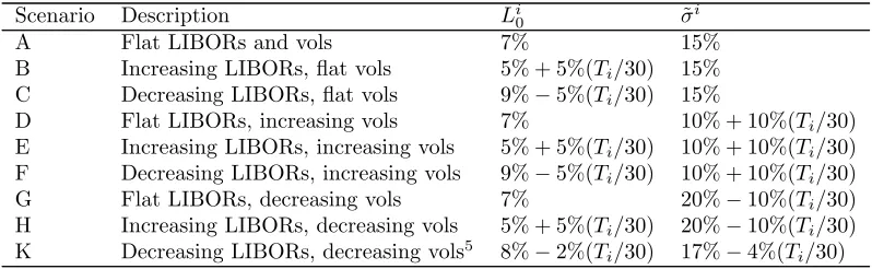
The market scenarios considered in our numerical study are detailed in Table 1. The tenor structure is taken to be annual with n = 29, thus T1 =

1, T2 = 2, . . . , Tn = 29, with final maturity Tn+1 = 30. In our specification

of the common driving process the mean reversion parameter a is taken to be 5% (see Section 4.1). However we have also examined results for other values of a_∈(0,20%) and find they are consistent with our conclusions.

4_{For the market model and drift approximation model this is immediate sinceL}n has zero drift (see equation (7)). Under the Markov-functional model this holds by definition at Tn (see equation (15)). At earlier times we may recover the relationship between L

n and xby applying the martingale property toLn

Scenario Description Li

0 σ˜

i

A Flat LIBORs and vols 7% 15%

B Increasing LIBORs, flat vols 5% + 5%(Ti/30) 15% C Decreasing LIBORs, flat vols 9%−5%(Ti/30) 15%

D Flat LIBORs, increasing vols 7% 10% + 10%(Ti/30) E Increasing LIBORs, increasing vols 5% + 5%(Ti/30) 10% + 10%(Ti/30) F Decreasing LIBORs, increasing vols 9%−5%(Ti/30) 10% + 10%(Ti/30) G Flat LIBORs, decreasing vols 7% 20%−10%(Ti/30) H Increasing LIBORs, decreasing vols 5% + 5%(Ti/30) 20%−10%(Ti/30) K Decreasing LIBORs, decreasing vols5 _8%

−2%(Ti/30) 17%−4%(Ti/30) Table 1: Scenarios for initial LIBORsLi

0 and caplet implied

volatilities ˜σi _{considered in our numerical study.} 6

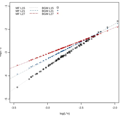
We first present our results under Scenario A, where initial LIBORs and caplet implied volatilities are flat, since these are typical of the results across all scenarios. The lines shown on Figure 1 display the functional relationship between a selection of LIBORs Li _{and the terminal LIBORL}n_{under the}

LI-BOR Markov-functional model at T15.The drift approximation model could

not be distinguished from the Markov-functional model on this plot and so is not shown. It is striking that the scatter plot overlaid of the corresponding market model simulation exhibits very little dispersion. We observe the plots are very close to a straight line (on a log-log scale) under both the Markov-functional and market models, for all exercise dates and scenarios. As an approximate measure of the linearity of these plots we consider the value of the statistic R2 _{computed using a large number of points; for this exercise}

5_{The scenario for decreasing rates and implied volatilities has been adjusted to ensure}

that the approximationξtis strictly increasing for allt(see Section 4.1).

6_{Under the market model and associated drift approximation model we require values of}

initial LIBORs and implied volatilities at times other thanT1, ..., Tn+1in the computation

date all plots have an R2 _{of at least 0.999 (indicating they are extremely}

close to straight lines).7

In general under Scenario A there is a close match between slopes and intercepts corresponding to the Markov-functional model and those of the least squares linear regression computed from the separable LIBOR market model simulation (results for T15 are given in Table 2). For a given exercise

dateTk,the slopes corresponding to the Markov-functional model tend to be

slightly higher than for the market model; the greatest difference generally occurs for LIBORs Li _{where i lies midway between k and n (at T}

15 this

occurs for L23_{). Note that under all models the relationship between L}k Tk and Ln

Tk under F is constrained to some extent by fitting to the kth Black’s caplet price. In addition, the terminal LIBORLn_{is exactly lognormal under}

F. Therefore, if the market model exhibits little dispersion it is only for LIBORs Li _{with i between k and n that we would expect any significant}

differences between models.

The drift approximation model is very close to both the Markov-functional and market models (in terms of slopes and intercepts). In general we observe that the Markov-functional model appears to be slightly closer to the market model for LIBORs i close to k (at T15 this holds for L15, L16 and L17) and

the drift approximation is closer for the remainder.

Any small differences between slopes and intercepts increases with the maturity of the tenor structure under consideration. These slopes and in-tercepts match to at least 3 s.f. for a maturity of 10Y, whereas we begin to observe small numerical differences for longer maturities (matching only to 2

7_{That is, the proportion of the variance in observations explained by a linear}

log(L^n)

log(L^i)

-3.5 -3.0 -2.5 -2.0

-5

-4

-3

-2

-1

MF L15 MF L21 MF L27

BGM L15 BGM L21 BGM L27

Figure 1: Graph of log(Li

T15) vs. the terminal LIBOR, log(L

29

T15),for a selection of

forward ratesi,assuming flat initial LIBORs and implied volatilities (Scenario A). Lines show the functional relationship under the Markov-functional (MF) model. Scatter plots overlaid give an indication of the relationship under the corresponding separable LIBOR market model (BGM).

LIBOR Log-linear MF BGM DA

Slopes L15 2.01 1.84 1.88 1.84

L21 1.49 1.51 1.45 1.44

L27 _{1.11 1.14 1.10 1.10}

Intercepts L15 _{1.9 2.0 1.9}

L21 _{1.3 1.1 1.1}

L27 0.4 0.2 0.2

s.f. at 20Y). These small differences may lead to minor differences in deriv-ative prices calculated under each model; these are discussed with reference to the example of the standard Bermudan swaption in Section 4.3.

This analysis of the relationship between LIBORs for various times Tk

has been repeated under all scenarios given in Table 1. The qualitative observations detailed above are found to hold under all scenarios. The same conclusions are also reached under a scenario corresponding to typical USD market data.8

The linearity of the market model’s scatter plot is perhaps surprising, as one might reasonably expect the model to produce more dispersion because the drift term is stochastic for LIBORs i < n. These plots indicate that the stochastic component of the drift remains small, hence although the market model is theoretically Markovian only in n dimensions, it generally resembles a one-dimensional model for all practical purposes. We take up this discussion again in Section 4.4, where we observe that for high volatilities and long maturities this is no longer the case and the market model plot exhibits much greater scatter.

As a means of understanding the trends in slopes of the three models it is convenient to contrast their behaviour with the following log-linear model. Since we have observed that the relationship between log(Li

t) and log(Lnt)

is close to linear, it follows that Li

t is approximately lognormal under F.

Therefore, suppose

log(Lit)≈η i t+c

i

xt =ηti+c i

Z t

0

σudWu

under F for some constant ci _{and a deterministic function of time η}i t. Note

that this model will admit arbitrage since otherwise we would require ηi t

to be stochastic. Now Var(log(Li

t)) ≈ (ci)2ξt, hence (ci)2ξTi ≈ (˜σ

i₎2_T

i by

matching terminal variances (since we are calibrating our model to caplet prices). Comparing with the separable volatility structure of the analogous LIBOR market model, ci

≈γi_.Thus,

log(Li t)≈

γi

γn

log(Ln t) + ˆηti

for some deterministic ˆηti. This is a coarse approximation to the LIBOR

market model and the corresponding LIBOR Markov-functional model but the slopes of this log-linear model are certainly comparable with the actual slopes observed under these models (matching to at least 1 s.f.; see Table 2). The approximation provides a good guide to trends expected in slopes of the log-log plots. For example, when ξTi is specified according to our Hull-White approximation (20), then γi _{is decreasing with i for flat caplet volatilities}

(see equation (21)). Therefore, it is not surprising that we see decreasing slopes on the associated log-log plots (see Figure 1).

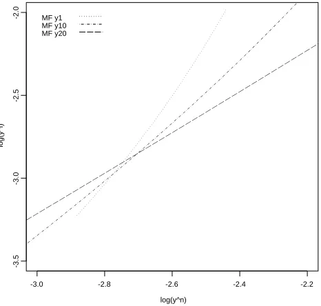
We now consider the functional forms of the co-terminal forward par swap rates yi

Ti (corresponding to swaps with fixed maturity Tn+1) implied by the one-factor LIBOR Markov-functional model. Subsequently, in Section 5 we perform a similar examination of the functional forms of LIBORs Li

Ti under the swap-based Markov-functional model.

Functional relationships between log(yi

Ti) and log(y

n

Ti) under Scenario A are displayed in Figure 2 for a selection of forward rates i.9 _{These functional}

forms are typical in that the numerical relationship appears to be close to linear, with slight positive convexity. This convexity is anticipated since par swap rates are a linear combination of lognormal forward rates, hence cannot also be lognormal.

9

Note that the terminal par swap rateyn

log(y^n)

log(y^i)

-3.0 -2.8 -2.6 -2.4 -2.2

-3.5

-3.0

-2.5

-2.0 MF y1 MF y10 MF y20

Figure 2: Typical graph of the functional relationship between a selection of co-terminal forward par swap rates log(yi

Ti) and the terminal forward rate log(y

29

Ti)

4.3

Example application:

Pricing a Bermudan swaption

It is clear from the numerical results above that for typical market data the LIBOR Markov-functional model is very close to the separable LIBOR mar-ket model with the same driving process, especially for short maturity tenor structures. Therefore we would also expect prices of exotic derivatives under the two models to be similar because these prices are effectively summary statistics. We demonstrate this with the example of a standard Bermudan swaption.

In common with most exotic derivatives with early exercise features, it is very difficult to price a standard Bermudan swaption directly using a sim-ulation of the market model. It is necessary to introduce further approxi-mations to determine the optimal exercise boundary. In theory, simulation-based methods such as the least-squares approach suggested by Longstaff & Schwartz [2001] can be used to compute the exercise boundary to any required accuracy but considerations of computation time must be taken into account. In contrast with the market model, the arbitrage-free Markov-functional model permits an efficient implementation as it stands, without the need for approximation.

Suppose we wished to price Bermudan swaptions in a model in which LIBORs are lognormal (this may be to mirror the behaviour of the LIBOR market model or to avoid negative LIBOR rates, for instance). In practice, we would need to choose the driving processxand market model parameters

γi _{carefully to reflect the appropriate joint distributions of rates (for example,}

correlation structure of all models is as described in Section 4.1 with mean reversion parameter a = 5%.

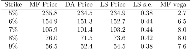
In Tables 3-5 we display a summary of prices of annual Bermudan swap-tions (7% payers swapswap-tions) with various maturities under the one-factor LIBOR Markov-functional (MF) model and the corresponding drift approx-imation (DA) model. Also included are Longstaff-Schwartz (LS) prices com-puted by direct simulation of the separable LIBOR market (SLM) model. A single explanatory variable (the current swap net present value) was used in the LS algorithm to determine the exercise boundary of the Bermudan swaption (via a simple linear regression across all in-the-money sample paths at each exercise date). Including further explanatory variables, which should theoretically improve the approximation to the exercise boundary, was not found to increase prices significantly. This observation may also be found in Pelsser et al. [2004] and Pelsser & Pietersz [2004]. The prices shown correspond to flat initial LIBORs and flat implied volatilities (Scenario A), however the results are found to be very similar over all scenarios.

Strike MF Price DA Price LS Price LS s.e. MF vega

5% 123.0 123.0 123.0 0.19 0.6

6% 73.1 72.9 73.0 0.18 2.0

7% 41.4 41.2 41.3 0.16 2.8

8% 24.0 23.9 24.0 0.13 2.7

9% 14.4 14.3 14.4 0.10 2.2

Table 3: 10Y annual Bermudan swaption prices (in basis points) under the Markov-functional model (MF) and the corresponding SLM model computed using both Longstaff-Schwartz (LS) and drift approximation (DA).

Strike MF Price DA Price LS Price LS s.e. MF vega

5% 197.0 196.6 196.6 0.30 1.7

6% 124.8 123.5 123.8 0.33 4.5

7% 80.6 79.0 79.4 0.32 5.7

8% 54.4 53.0 53.3 0.29 5.7

9% 38.1 36.8 37.3 0.25 5.2

Table 4: 20Y annual Bermudan swaption prices.

Strike MF Price DA Price LS Price LS s.e. MF vega

5% 235.8 234.5 234.9 0.38 2.7

6% 154.9 151.3 152.7 0.44 6.5

7% 105.9 101.4 103.2 0.44 8.0

8% 76.0 71.5 73.6 0.42 8.0

9% 56.5 52.4 54.5 0.38 7.6

At 20Y, slight price differences are observed between the (arbitrage-free) SLM and MF models in all scenarios. The MF model gives consistently higher prices especially for out-of-the-money options. Recall from section 4.2 that the slopes and intercepts of the log-LIBOR plots do not match to such high accuracy at 20Y, though it is clear from the distributional study that the models remain very similar qualitatively. It is arguable that in practice these price differences would not be considered large (they are consistently well below the MF vega). Prices under the DA model are reasonably close to LS but are systematically lower. This may be of concern since the LS price is theoretically a lower bound for the true Bermudan price under the SLM model (since the exercise strategy may theoretically be improved).

At 30Y, the price differences increase across all scenarios. Again DA prices are observed to be below LS prices, which in turn lie below MF prices. The numerical error between LS and DA prices is still small in comparison with MF vega; the maximum difference is approximately half the vega. From a practitioner’s viewpoint, it is arguable that this model error is still acceptable, being within what would be taken in profit, though it is clear the observed differences could represent a large proportion of that profit.

Numerical accuracy is important in determining the LS price. To achieve convergence to the desired accuracy 100,000 paths were required (50,000 plus 50,000 antithetic), each with 100 time steps between each exercise date. Using fewer time steps introduces discretisation error that may affect the Bermudan price at this accuracy.10 _{As the MF model remains qualitatively}

similar to the SLM model its efficient implementation would appear to be preferable.

10_{This could be remedied by, for example, applying a predictor-corrector approximation}

It is anticipated that including the smile in implied volatilities (in this one-factor setting) will have a much larger impact on prices than these model differences, since this will change the functional forms significantly. This is illustrated by Pelsser & Pietersz [2004], who note similarities in Bermudan prices between the MF and SLM models that both exhibit displaced diffusion dynamics. A version of the uniqueness result can still be formulated in this situation; this would certainly help explain the similarity between the models in the one-factor case.

4.4

Stress testing

In this subsection the three LIBOR models are compared under more un-usual market conditions. We find that it is the presence of high volatilities that has a significant impact on the match between models. Results of the distributional study are presented only for a maturity of 30Y because for shorter maturities the effect is far less noticeable. The effects of stressing the values of initial LIBORs for reasonable volatility levels have also been examined but the consequences are relatively insignificant.

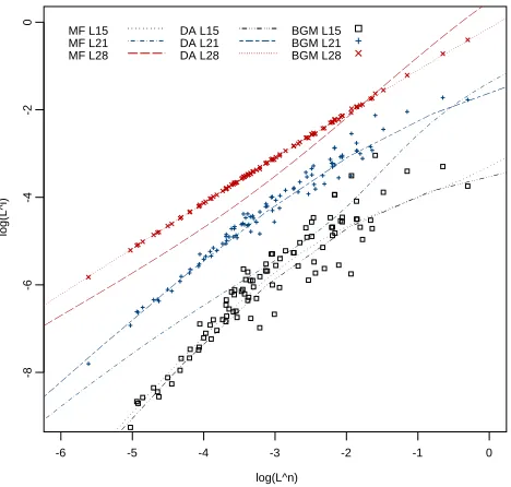
The impact of high volatilities is clearly illustrated in Figure 3, where we plot log(Li

T15) against log(L

n

T15) for extremely high implied volatilities of 50%. Under the market model, the linear relationship previously observed between log(Li

Tk) and log(L

n

Tk) breaks down. Also the points of the scatter plot are more widely spread out, hence the market model can no longer be well represented by a single functional form.

log(L^n)

log(L^i)

-6 -5 -4 -3 -2 -1 0

-8

-6

-4

-2

0

MF L15 MF L21 MF L28

DA L15 DA L21 DA L28

BGM L15 BGM L21 BGM L28

Figure 3: Plot of log(Li

T15) vs. log(L

n

T15) for initial LIBORs of 7% and very

model and the drift approximation model may give rise to very different func-tional forms even when the market model exhibits little dispersion at a given exercise date. This can be seen for example by looking at the plots forL28

T15 in Figure 3 and is further illustrated below by increasing mean reversion. Note that under the conditions of Figure 3 the drift approximation model begins to exhibit significant arbitrage and the effects of this are not immediately clear (see discussion below).

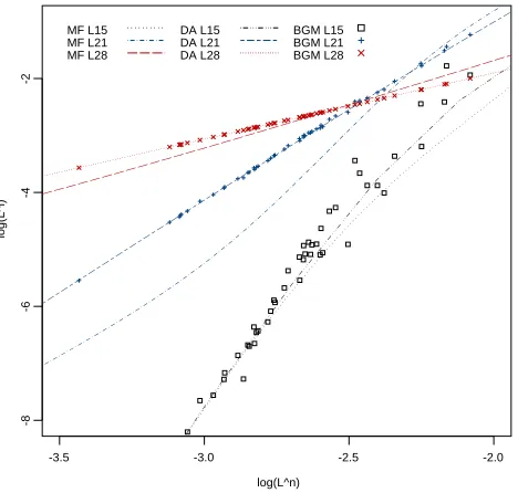
Figure 4 displays the same results as given in Figure 3 for a higher value of the mean reversion parameter (a= 15%). Consider the plots ofL21

T15 under each model. The presence of high mean reversion means that the common instantaneous volatility function σ increases steeply over successive time in-tervals. This results in the constantsγi_{, chosen via equation (21), decreasing}

dramatically as iincreases. Therefore, under the market model the stochas-tic component of the integrated drift terms appearing in the expression for

L21

T15, which contains a (γ

i₎2 _{term, will dominate the non-stochastic}

compo-nent of the drift, which only contains terms γi_γj_{, j > i (see equations (8)}

and (9)). Thus, the scatter plot of the market model simulation exhibits little dispersion at T15.For the same reason, the standard application of the

Brownian bridge drift approximation to this market model gives a functional form that lies close to the scatter plot. In contrast, the functional form of

L21

T21 under the Markov-functional model is typically very close to the corre-sponding market model plot atT21but may differ at earlier times; we observe

significant differences atT15.As we explain below, this is because these

func-tional forms are computed iteratively, backwards through time, by applying the martingale property (14).

no-log(L^n)

log(L^i)

-3.5 -3.0 -2.5 -2.0

-8

-6

-4

-2

MF L15 MF L21 MF L28

DA L15 DA L21 DA L28

BGM L15 BGM L21 BGM L28

Figure 4: The same set of results for high volatilities as displayed in Figure 3 but

ticeable arbitrage in the drift approximation model. In order to ensure the implementation of any model is arbitrage-free in practice, we require that the martingale property of numeraire-rebased discount factors is numerically sufficiently accurate at all times. This is far from true for the drift approxima-tion model under these unusual circumstances, as we show below. Accuracy of the martingale property is essential for pricing Bermudan-style derivatives since it is implicitly assumed when computing the time value of a derivative (the value of continuation) at a given exercise date (for a Bermudan swap-tion this is the maximum of the expectaswap-tion under F of the payoff at the subsequent exercise date and the value of immediate exercise).

A practical implementation of the drift approximation model may of course be constructed by assuming the functional forms of Li

Ti are taken to be those given by the usual drift approximation model for 1_≤i_≤n and recovering the remaining functional forms of Li

Tj at exercise dates Tj < Ti using the martingale property of numeraire-rebased discount factors (14).11

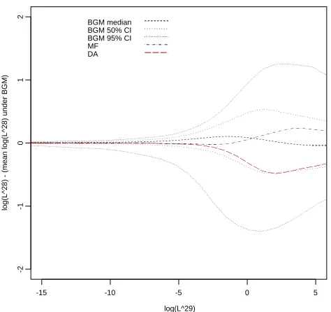
In our example, the terminal LIBOR L29 is a known analytic function of x

at all times. If L28

T28 is assumed to be given by the drift approximation as usual, then L28

T27 may be recovered by applying the martingale property. Figure 5 allows us to compare the functional forms of logL28

T28 under both the Markov-functional model and the drift approximation model constructed using the martingale property. In displaying these functional forms, for each value of the terminal LIBOR L29

T28 we have simulated the market model con-ditional on this value and subtracted the mean value of logL28

T28 under this model from each of the functional forms. Confidence intervals under the mar-ket model for the value of logL28

T28 conditional on the value of L

29

T28 are also

11

provided. It appears that the functional form of logL28

T28 under the Markov-functional model is closer to the mean value of logL28

T28 under the market model (given L29

T28) than under the drift approximation model.

log(L^29)

log(L^28) - (mean log(L^28) under BGM)

-15 -10 -5 0 5

-2

-1

0

1

2

BGM median BGM 50% CI BGM 95% CI MF DA

Figure 5: Plot of log(L28

T28) minus the mean value of log(L

28

T28) conditional on

the value ofL29_T28 under the separable LIBOR market model, against the terminal LIBOR, log(L29_T28).

Given this observation, it is reasonable to expect that when applying martingale property to compute the values ofL28_{at earlier exercise dates the}

Markov-functional model will be closer to the market model than the drift approximation model. This is confirmed by Figure 6, which shows a typical LIBOR functional form computed by applying the martingale property to the drift approximated LIBORs L28 _{at the previous exercise date T}

27. This

arbitrage-free under these extreme circumstances, then in general it is the Markov-functional model that appears to be closer to the market model than the drift approximation model.

log(L^n)

log(L^i)

-12 -10 -8 -6 -4 -2 0 2

-20

-15

-10

-5

0

5

MF L28 DA L28 BGM L28

Figure 6: Plot of log(L28_T27) vs. the terminal LIBOR, log(L29_T27). Here the drift approximation plot (DA) is calculated by applying the martingale property to the functional form ofL28

T28 that is computed under the drift approximation model (see

Figure 5).

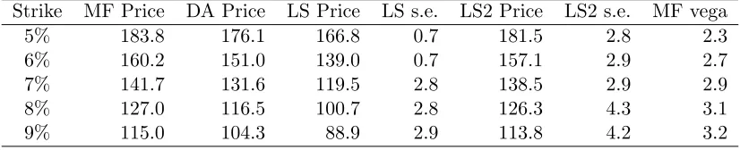
We conclude this section with a brief discussion of Bermudan swaption prices under this unusual scenario (see Table 6). Generally, the standard error in the Longstaff-Schwartz price is very large; this is not surprising be-cause simulated Bermudan prices are likely to be much more spread out if implied volatilities are very high. For 30Y, the standard error is so large (approx 220 bps for 100,000 paths), it renders the method practically use-less without much more sophisticated variance reduction methods. For all maturities, including a second explanatory variable (the current LIBOR) in the least-squares regression at each step increases the Bermudan price signif-icantly (these prices are denoted by ‘LS2 Price’ in Table 6). This is because under these market conditions the separable LIBOR market model is no longer well represented by a one-dimensional model (with the correspond-ing one-dimensional exercise boundary). It is possible that includcorrespond-ing further explanatory variables in the regression may increase the price still further. The MF prices consistently remain very close to the centre of the 95% LS2 confidence interval, whereas the DA price is typically below the lower 95% confidence limit. This example illustrates how any approximation to the LIBOR market model may break down in unusual circumstances even if it performs well in the majority of situations.

Strike MF Price DA Price LS Price LS s.e. LS2 Price LS2 s.e. MF vega

5% 183.8 176.1 166.8 0.7 181.5 2.8 2.3

6% 160.2 151.0 139.0 0.7 157.1 2.9 2.7

7% 141.7 131.6 119.5 2.8 138.5 2.9 2.9

8% 127.0 116.5 100.7 2.8 126.3 4.3 3.1

9% 115.0 104.3 88.9 2.9 113.8 4.2 3.2

5

Numerical comparison of swap models

In this section we report the results of a similar numerical study of the anal-ogous relationships between rates under the swap market model,12 _the

asso-ciated swap drift approximation model and the corresponding swap Markov-functional model with the same driving process.

The construction of a swap Markov-functional model that closely matches the swap market model considered in Section 2.4 is analogous to that for the LIBOR case. As in the swap market model we assume a set of co-terminal forward par swap rates, denoted by yi _{for i = 1, .., n. The ith forward par}

swap rateyi _{sets on dateT}

i with coupon payments on datesTi+1, ..., Tn+1 and

satisfies (11). We assume that the market prices for the vanilla swaptions on the ith swap rate are given by Black’s formula. The driving Markov process and the choice of numeraire are exactly as in the LIBOR case but now it is the ith forward par swap rate at time Ti, yTii, which is assumed to be a monotonic increasing function of the variable xTi.

The numeraire bond at timeTn, DTnTn+1(xTn),is chosen exactly as for the LIBOR model. However the functional form for the numeraireD·Tn+1at times

Ti, i= 1, ..., n−1,needs to be determined. The reader is referred to Hunt &

Kennedy [2000] for the full details of the calibration step, this time carried out using synthetic PVBP-digital swaptions as the calibrating instruments. The algebra involved in these intermediate steps is no more onerous than for the LIBOR-based Markov-functional model (whereas the drift term of the swap market model is found to be more complex than in the LIBOR market model). The reader will note that a similar uniqueness statement to that given in Section 3.3 can be formulated for the swap Markov-functional model.

In the following, the driving process x of the swap Markov-functional model is taken to be of the same form as for the LIBOR-based model but the variances of x at each Ti are now chosen by considering a Hull-White

model calibrated to at-the-money European swaption prices (see Appendix A). Linear interpolation is used to complete the specification of the swap-based market model. The mean reversion parameter is taken to be a = 5%.

The tenor structure under consideration is taken to be the same as for the LIBOR case.

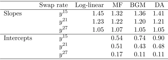
Our conclusions are very similar to those for the analogous LIBOR-based models for the scenarios in Table 1. We observe that log(yi

Tk) is approxi-mately linear in log(yn

Tk) for all models and that the slopes and intercepts agree to high accuracy (see Table 7 for the case of flat initial LIBORs and implied caplet volatilities (Scenario A)). Note that the accuracy of approxi-mations suggested in Pelsser & Pietersz [2004] for the calibration of a swap Markov-functional model to a swap correlation matrix (either market-implied or historically estimated) is easily explained by the linearity of this relation-ship, since this means the Taylor expansion of log(yi

Tk) about xTk to order one is almost exact. Approximations along the same lines could be derived to aid calibration of the LIBOR Markov-functional model by observing the lin-earity of the corresponding relationship between log LIBORs and the driving process under the LIBOR model.

In exploring the functional forms of the forward LIBORsLi

Swap rate Log-linear MF BGM DA

Slopes y15 _{1.45 1.32 1.36 1.41}

y21 _{1.23 1.22 1.20 1.21}

y27 1.05 1.07 1.05 1.05

Intercepts y15 0.54 0.74 0.90

y21 0.51 0.43 0.48

y27 _{0.17 0.11 0.11}

Table 7: Slopes and intercepts of functional forms of for a selection of (log) forward

par swap rates at T15 under the Markov-functional model (MF), drift

approxima-tion (DA) and the log-linear approximaapproxima-tion. Also shown are slopes and intercepts of the least squares linear regression fitted to the corresponding swap market model (BGM) results.

log(L^n)

log(L^i)

-6 -5 -4 -3 -2 -1

-10

-8

-6

-4

-2

MF L1 MF L10 MF L20

Figure 7: Forward LIBOR functional forms under the swap-based Markov-functional model: Plot of log(Li

Ti) vs. log(L

n

Ti) for a selection of forward LIBORs

LIBORs. Functional forms are truncated for negative values of Ln

Ti in the graph shown.

6

Conclusion

In this paper we have explored the relationship between LIBORs under the one-factor LIBOR market model with separable volatility structure and the corresponding one-factor Markov-functional model. We have observed that for short maturities (10Y) these models are numerically equivalent for all practical purposes under a wide range of market conditions. For longer ma-turities, slight differences are observed in our distributional study, however the models remain qualitatively similar. Therefore, much of the intuition of the familiar SDE formulation of the separable market model may be applied in the specification and calibration of the Markov-functional model. As ex-pected given the close match between models at 10Y, the prices of exotic derivatives such as Bermudan swaptions under these models are practically identical. For longer maturities, it is possible to distinguish between prices, however it is arguable that the difference is not material from a practical perspective. In this case, the straightforward efficient implementation LI-BOR Markov-functional model may be preferable to any time-consuming simulation-based implementation of the LIBOR market model. It is also preferable to the drift-approximation model because it is guaranteed to be arbitrage-free.

the drift approximation model now exhibits noticeable arbitrage and conse-quently it may lead to inaccurate derivative prices. In contrast, the LIBOR Markov-functional model remains qualitatively similar to the LIBOR market model and may therefore be considered a more appropriate choice of pricing model. Considering again the example of the Bermudan swaption, it appears that prices under these two models remain consistent under this extreme sce-nario, whereas the drift approximation model tends to lead to a significant underpricing. Our results highlight the dangers of using an approximation to an arbitrage-free model where the limitations of the approximation are not fully understood.

In a separate line of discussion, the behaviour of functional forms of for-ward LIBORs under the swap-based Markov-functional model are found to be somewhat unrealistic for long maturities (where in some cases LIBORs may become negative). This is an artefact common to all one-factor swap rate based models. In contrast, the behaviour of forward par swap rates under the LIBOR Markov-functional is found to be as expected.

References

Andersen, L. & Andreasen, J. [2000], ‘Volatility skews and extensions of the LIBOR market model’, Applied Mathematical Finance 7(1), 1–32.

Brace, A., G¸atarek, D. & Musiela, M. [1997], ‘The market model of interest rate dynamics’, Mathematical Finance7(2), 127–155.

Carverhill, A. [1994], ‘When is the short rate Markovian?’, Mathematical

Finance 4(4), 305–312.

Hull, J. & White, A. [1990], ‘Pricing interest rate derivative securities’, The

Review of Financial Studies 3(4), 573–592.

Hunt, P. J., Kennedy, J. E. & Pelsser, A. A. J. [2000], ‘Markov-functional interest rate models’, Finance and Stochastics 4(4), 391–408.

Hunt, P. & Kennedy, J. [2000], Financial derivatives in theory and practice, John Wiley & Sons, Chichester.

Hunt, P. & Kennedy, J. [2005], ‘Longstaff-Schwartz, effective model di-mensionality and reducible Markov-functional models’. Working Paper (available from www.ssrn.com).

Hunter, C., J¨ackel, P. & Joshi, M. [2001], ‘Getting the drift’, Risk Magazine

(July).

Jamshidian, F. [1997], ‘LIBOR and swap market models and measures’,

Fi-nance and Stochastics 1, 293–330.

Kurbanmaradov, O., Sabelfield, K. & Shoenmakers, J. [2002], ‘Lognormal approximations to LIBOR market models’, Journal of Computational

Longstaff, F. & Schwartz, E. [2001], ‘Valuing american options by simula-tion: A simple least-squares approach’,The Review of Financial Studies 14(1), 113–147.

Milterson, K., Sandmann, K. & Sondermann, D. [1997], ‘Closed form so-lutions for term structure derivatives with log-normal interest rates’,

Journal of Finance 52(1), 409–430.

Pelsser, A. & Pietersz, R. [2004], ‘A comparison of single-factor Markov-functional and multi-factor market models’. Working Paper (available from www.few.eur.nl/few/people/pelsser).

Pelsser, A., Pietersz, R. & van Regenmortel, M. [2004], ‘Fast drift-approximated pricing in the BGM model’, Journal of Computational

A

Approximating the Hull-White correlation

structure

In this appendix we specify the driving processxby deriving an approximate expression for the variance

ξTi := var(xTi)

of xat timesTi, i= 1, ..., n.This approximation is arrived at by considering

a Vasicek-Hull-White model calibrated to at-the-money caplet prices in the LIBOR case and at-the-money European swaption prices in the swap case.

Consider a Hull-White model in which the short-rate processrsolves the SDE

drt = (θt−art)dt+ ˆσtdWct,

where a is a constant, θ and ˆσ are deterministic functions of t and cW is a standard Brownian motion under the risk-neutral measure Q. For 0 _≤ t _≤ Tn+1 the measures Fand Qare related by

dF dQ Ft = exp − Z t 0

rudu

DtTn+1

D0Tn+1

.

Let x be defined as in equation (10) and define ˆσt=e−atσt. Working in the

measure F it is straight forward to derive an analytical expression for the functional forms ˆDtTi(xt), i= 1, ..., n. We find

ˆ

DtTi = ˆD0Tiexp

(ψTn+1−ψTi)xt− 1

2(ψTn+1−ψTi)

2_ξ

t

, (22)

where

ψt:=

1

a(1−e

−at_),

and

ξt :=

Z t

0