Long term morphodynamic behaviour of the Maasvlakte 2 sand extraction pits and the influence on surrounding sand wave fields

Long-term morphodynamic behaviour of

the Maasvlakte 2 sand extraction pits

and the influence on surrounding

sand wave fields.

MSc Thesis in Civil Engineering and Management Britt de Groen

Long-term morphodynamic behaviour of the

Maasvlakte 2 sand extraction pits and the

influence on surrounding sand wave fields.

Student:

Location and date: Thesis defense date:

Graduation supervisor:

Daily supervisor:

External Supervisors:

Britt de Groen BSc. Enschede, March 26, 2015 April 2, 2015

Prof. dr. S.J.M.H. Hulscher

(University of Twente)

Dr. ir. B.W. Borsje

(University of Twente) (University of Twente)

Dr. ir. P.C. Roos

(University of Twente)

Ir. T. Ligteringen

(Royal Netherlands Navy)

Drs. A. Stolk

(Ministry of Transport, Public Works and Water Management)

MSc thesis in Civil Engineering and Management

Faculty of Engineering Technology

Voorwoord

Hier voor u ligt de afstudeerscriptie, waar ik het laatste half jaar aan gewerkt heb. Met het be¨eindigen van dit project rond ik ook het laatste deel van mijn studie af. Het project over de zandwinputten van de tweede Maasvlakte heb ik met plezier gedaan. Zowel het technisch als het praktische aspect kwamen er beide in voor. Dit zorgde voor afwisseling in de opdracht en heeft er toe geleidt dat ik veel verschillende mensen heb ontmoet.

Ik wil Leendert en Ad bedanken voor de mogelijkheid die ze mij gegeven hebben om het onder-zoek uit te voeren, maar vooral voor de kritische houding en de focus op het praktische gedeelte. Daarnaast wil ik Suzanne bedanken voor de feedback gesprekken en dat ik mee mocht naar de leerzame en gezellige NCK dagen!

Bas, bedankt voor je enthousiasme, je relativeringsvermogen en je Matlab-skills. Je hebt me enorm geholpen met aandachtig te kijken naar data, niet te stressen en vaak heb je me een glimlach bezorgd. Bedankt!

Pieter, jou wil ik bedanken voor je geduld en de hulp met het model. Je feedback was altijd duidelijk en kon altijd bij je binnen lopen, dat was heel fijn.

Thijs, je hebt me eeen kijkje gegeven in de wereld van de Marine, wat voor mij geheel onbekend was. Bedankt voor de leuke en leerzame gesprekken, je hebt ervoor gezorgd dat ik me de dagen in Den Haag erg op me gemak voelde!

Daarnaast wil ik de Dienst der Hydrografie bedanken voor de leuke gesprekken en vaste lunch-pauzes, het waren fijne weken! Dani¨elle bedankt voor de wondere wereld van de bathymetrie, je enthousiasme en hulp, waar ik maar vragen kon! Martien bedankt voor je kritische kijk op mijn scriptie en de gezellige koffie momenten! John, bedankt voor een onvergetelijk weekend op de Luymes, het was geweldig!

De studenten in de afstudeerkamer wil ik graag bedanken voor het accepteren van een chaotisch bureau en daarnaast voor de oneindige wandelingen richting het koffiezetapparaat.

Lieve vrienden, bedankt voor de fantastische jaren die ik in Enschede heb mogen meemaken. Bedankt voor de vriendschap, gezellige avonden en gesprekken, zonder jullie was het een saaie boel geweest!

Lieve Leonie, bedankt voor een fijne thuishaven en dat je altijd voor me klaar staat, vooral tij-dens de laatste loodjes.

Tot slot wil mijn lieve ouders bedanken, voor de mogelijkheid die ze mij gegeven hebben om te studeren en mezelf te ontwikkelen. Ik kan jullie niet beschrijven hoe erg ik dat waardeer en hoeveel liefde jullie mij geven.

Last but not least, wil ik Tycho bedanken, voor je positiviteit, hele fijne weekenden en je geduld. Je bent de liefste en nu is het tijd voor onze toekomst samen, ik ben er klaar voor!

Liefs, Britt Maart, 2014

Abstract

The Rotterdam harbour is one of the largest harbours in the world and still expanding. The most recent expansion is called Maasvlakte 2 (MV2), which added 2000 hectares to the west of the existing port into the sea. MV2 was realised between 2009 and 2013 using sand dredged some kilometres o↵shore in the North Sea. A total of 200 million m3 sand was extracted from two sandpits with volumes of 170 Mm3 and 30 Mm3 . Those sandpits are located nearby the navigation channel to Rotterdam and surrounded by sand wave fields. Since sand waves have a migration rate in the order of 5 meters per year and a height of 5 meters, they can hinder navigation. Therefore it is important to know how sand wave fields behave. The purpose of this study is to determine the long-term e↵ects of the sandpits of Maasvlakte 2 on the surrounding sand wave fields.

This is study is done by a data analysis of bathymetric data and secondly a model study for the long-term behaviour of sand pit and the sand wave fields. The bathymetric data is gathered from the anchorage area, a sand wave field 6 km away of the sand pits. These bathymetric data is analysed by a Fourier analysis (van Dijk et al. 2006) to calculate the specific sand wave characteristics. With a linear regression method the migration rate is determined for the sand waves. This is done for the period between 2006 and 2014, divided into two stages, one before and one after the realisation of the sandpits.

The sand waves show a dynamic migration rate, with a range between 4.0-5.8 m/year. Before the realisation of the sandpit the range was between 3.9- 6.9 m/year and in the after stage a range of 2.6- 5.8 m/year. Because the calculation of these migration rates is very dependable of the place and angle, there cannot be made a conclusion based on this results.

Modelling the long-term behaviour is done in two steps: (i) by modelling the sandpit in an idealized morphodynamic model (Roos et al. 2008) and, (ii) to use these results as input for a smaller-scale idealized sand wave model (Besio et al. 2006). The sandpit model is forced by tidal flow conditions as they apply near the sandpits, and the sandpit geometry is taken from recent surveys.

Next, a simulation is carried out indicating how the pit will deform and migrate over the next century. Throughout this evolution, and at fixed locations, the tidal flow pattern and local depth can be extracted. This flow pattern and local depth are used as local forcing for the smaller-scale

wave characteristics such as wavelength, orientation, growth and migration rates. Being driven by the gradually changing flow conditions and depth from the sandpit model, it indicates how the sand wave characteristics are a↵ected by pit evolution.

The models show the following long-term behaviour of the sandpits: The edges will flatten out, the little pit will move to the larger sandpit and the pits will move with the dominant flow direction. When the navigation channel is also implemented into the model, the ridge between the pits and the channel will gradually vanish. This eventually results in one large pit. The dredging activities of the channel are not taken into account in the model.

When looking again to the situation without the navigation channel, all sand wave fields surrounding the pits have crests with a north-east orientation. Those sand wave fields have the same response time as the Westhinder sand wave field, in the Belgium sea shelf. At the centre of the pit, sand waves will appear as well which have also crests with a north-east orientation. However, this orientation fluctuates with a small range throughout the years. If in reality there is silt present at the centre of the pit, which is most likely, no sand waves will arise.

It can be concluded that the sandpits do not have a large impact on their surroundings. This is positive for the navigation maintenance, because no large changes will be expected over time.

Contents

1 Introduction 1

1.1 Problem definition . . . 4

1.2 Research objective . . . 4

1.3 Methodology . . . 5

1.4 Reading guide . . . 6

2 Background information 7 2.1 Maasvlakte 2 . . . 7

2.2 Sandpit . . . 8

2.3 Sand waves . . . 9

2.3.1 Occurrence . . . 10

2.3.2 Sand wave theory . . . 10

2.3.3 Migration . . . 12

3 Bathymetric data study 13 3.1 Collecting bathymetric data . . . 14

3.1.1 Collecting devices . . . 14

3.2 Location of the bathymetric data study . . . 16

3.3 Bathymetric data analysing . . . 19

3.3.1 Method description to analyse the data . . . 19

3.3.2 Migration rates from bathymetric data . . . 24

4 Model set up 27 4.1 Sandpit model . . . 29

4.1.1 Description . . . 29

4.1.2 Input . . . 31

4.3 Output . . . 37

5 Results 39 5.1 Sandpit morphodynamic evolution . . . 39

5.2 Sand wave characteristics . . . 48

5.3 Practical application . . . 52

5.4 Comparison with the results of Svaˇsek . . . 56

6 Discussion 59 7 Conclusion 63 8 Recommendations 65 Bibliography 66 Appendices 69 A Bathymetric data analysis 71 A.1 Calculated sand wave characteristics . . . 72

A.2 Calculated sand wave migration rates . . . 73

B Calculation method on tides 75 B.1 Velocity output of the sandpit model . . . 78

B.2 Transform the velocity output of the sandpit model to input for the sand wave model . . . 79

C Results at the di↵erent positions 81

Chapter 1

Introduction

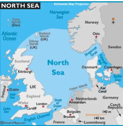
The landscape of the seabed changes by sedimentation and erosion, this is due to a storm or tidal currents. Because of the large changes it is important to study the marine-morphodynamics, es-pecially for the seabed. This study concentrates on the morphodynamic behaviour in the North Sea.

The North Sea is situated between The Netherlands, Germany, Denmark, Norway, United King-dom, France and Belgium (see Figure 1.1). A very busy shipping route is located in the southern part of this sea, which connects Northwest Europe to the rest of the world. Besides shipping, fishery, cables, pipelines, wind farms, gas-, sand- and oil extraction are important activities tak-ing place in the North Sea.

An important harbour in the North Sea is the mainport of Rotterdam. To enable economic growth an extension was needed. Therefore the second Maasvlakte was built as enlargement of the mainport. For this enlargement approximately 200Mm3 _{sand was needed. This sand was} extracted from the bed of the North Sea.

Figure 1.1: Location of the North Sea (source: home.comcast.net, 2014)

The amount of sand is dredged between 2008 and 2013 (Havenbedrijf Rotterdam, 2009). Mostly the maximum dredge depth is two metres, for this project an exception is made by Rijkswater-staat (Dijkshoorn and Stolk, 2009). Two sandpits arose with larger depths; a large sandpit with an area of 13.2 km2_{, a depth between 10-20 metres below the original sea bed and a volume of} 170Mm3_{and a smaller sandpit with a volume of 30Mm}3_{, an area of 2.6 km}2_{and a depth between} 10-12 metres below the original sea bed (Dijkshoorn and Stolk, 2009; Schipper, 2014).

There was not a lot experience with that amount of dredged sand, only with smaller amounts. For instance between 1996-2000, there were two pits created; the ’Drawing Pin’ pits and the PUT-MOR pit. The ’Drawing Pin’ pits were temporary sand extractions in the near shore coastal zone and were relatively deep - up to a maximum of 20 metres below the local sea bed elevation - with steep slopes. The ’Drawing Pin’ pits were located by Heemskerk/Wijk aan Zee (Hoogewoning and Boers, 2005). There was sedimentation in the pit and the slopes were slightly levelling of (Hoogewoning and Boers, 2001). The PUTMOR pit was a large-scale- and deep-extraction pit outside the coastal zone, located in the north of the Euro-Maas channel (Hoek van Holland) and research was executed to obtain more knowledge on sandpits with an extraction depth deeper than 2 metres. This sandpit had a volume of 4.5Mm3_{, with a surface area of 0.65 km}2 _{and a} depth varying between 5 and 12 metres (Boers, 2005). Svaˇsek (2001a,b,c) conclude with a field study that the influence of the sandpit on the flow velocities is generally small and that there was no morphological evolution visible in the measuring period.

3

Figure 1.2: Location of the sandpits and channels and the depth in meters. (2.Eurochannel, 1.Maaschan-nel, 3.turn-channel) [source: HNLMS Snellius, 2012]

1.1.

Problem definition

The behaviour of the sandpit in coastal environment strongly depends on the sediment supply, hydraulic conditions and orientation of the pit (Van Rijn and Walstra, 2004). Following Roos et al. (2008) a modelled sandpit with a volume of 48Mm3_{and a depth of 2 metres has an impact} on the morphological dynamics of the surroundings. The size of the impact depends on time, bottom friction, Coriolis and orientation of the pit with respect to the tidal flow. The realised sandpits from Maasvlakte 2 have a much larger depth, namely between 10 and 20 metres. Ac-cording to Klein and van den Boomgaard (2013), who studied the evaluation of the two sandpits with a hydraulic model, the sandpit will silt up and sharp edges will flatten over the years. These studies are based on hydrodynamic and morphological models. After the creation of the sandpits there are a lot of changes in the North Sea. These changes will cause dynamic changes in the surrounding area of the sand pit (for example: wave height, flow velocity etc.), where sand waves fields are situated. The normal sand wave migration rate in this area is 10 metres per year (Dorst, 2009), while the data study from Schipper (2014) shows a more dynamic migration rate.

For the navigation in the North Sea it is important to predict the behaviour of the sand wave fields. Because the ships have to take into account the place and height of the sand waves. The current problem is that there is no experience with large dimensions of a sand extraction pit, especially with a large depth. This has consequences on the morphodynamic behaviour, which influence the surroundings, where sand waves are present.

1.2.

Research objective

The objective of this thesis is to understand the morphodynamic behaviour of the sandpit and the influences of the surrounding sand wave fields.

Based on this objective, the following research questions are addressed:

- Which morphological behaviour in- and outside the sandpits is visible over 200 years? - Are there sand waves arising inside the pit?

1.3. Methodology 5

1.3.

Methodology

To study the research objectives, a methodology is used with several models. Because there is not a model which is capable to model the extracted sandpit and the occurrence of sand waves, the modelling approach is done in two steps.

To implement the sandpits an idealised morphodynamic model is used from Roos et al. (2008). This model has a little calculation time and is forced by tidal flow conditions near the sandpits. The simulation is carried out indicating how the pit will deform and migrate over time. At fixed locations the tidal flow patterns and depth can be extracted.

The model of Besio et al. (2006) is used to study the occurrence of the sand waves. This is a smaller-scale idealised model, with a linear stability to estimates the sand wave characteristics as wave length, orientation and growth rates. Also this model has a little calculation time and is forced by tidal flow conditions, grain size and water depth.

In order to achieve the research objective and to answer the research questions, the following methodology is used:

. Gathering bathymetric data to implemented the realised pits into the sandpit model. This is done by the Hydrographic Service of The Netherlands Navy, they gather data from hydrographic survey vessels and make nautical charts of these bathymetric data. . Analyse the quality of the bathymetric datasets in surrounding sand wave fields of the extracted sandpits. This is done by method of Van Dijk et al. (2008) which calculates the position and wave length of the sand waves. Finally with the calculated sand wave characteristics the migration is calculated.

. Next, the bathymetric data and the tidal flow conditions need to be transformed into an input for the sandpit model of Roos et al. (2008). After the transformation the model can be ran with the specific conditions for this case.

. With the output of the sandpit model the morphodynamic behaviour of the sandpits are visible. The model simulates the deform and migration of the sandpits by calcu-lating the local depth. This is done for the situation with- and without the extracting sandpits for the period 0 to 200 years.

. The local depth and flow conditions are calculated for fixed locations. Namely, the deepest depth in the pit, in the anchorage area, in a non-influenced area and at existing sand wave fields. This output can be used as input for the sand wave model of Besio et al. (2006). This model calculates if the circumstances are present for sand wave occurrence. When sand waves occur, the model calculates the characteristics as wave length and growth rate. With this information a conclusion can be made by the evolution of sand wave fields and if the characteristics are influenced by the realisation of the sandpit.

1.4.

Reading guide

Chapter 2 – Case description: a description of the Maasvlakte 2 and the basics of sand waves and sandpits.

Chapter 3 – Bathymetric data study: how are bathymetric surveys performed, the method of analysing the available data on specific locations and the calculations of the migration rate of sand waves.

Chapter 4 – Model description: description of the model from Roos et al. (2008) and Besio et al. (2006) and the used input and output of the models.

Chapter 5 – Results: the results of the morphological behaviour of the sandpits, the sand wave characteristics at di↵erent locations, the interaction between the sandpits and navigation channel and answers to the first and second research questions.

Chapter 6 – Discussion: discussions of the input of the models and the availability of bathymetric data.

Chapter 2

Background information

The North Sea is a dynamic area where many processes take place. In this chapter relevant background information is given about the second Maasvlakte and sandpits as well as extra information about sand waves.

2.1.

Maasvlakte 2

The Rotterdam harbour is one of the biggest harbours of the world and the biggest harbour in Europe (JOC, 2012). In 2004 the harbour of Rotterdam was beaten by Shanghai, to stay at a high position extension was needed (AAPA, 2004). The expanded harbour increased the economic value of the harbour, for now and in the future. The expansion of the Rotterdam harbour is called the Maasvlakte 2 and Figure 2.1 gives a representation of the present situation. Maasvlakte 2 is a location for port activities and industry, immediately to the west of the present port and industrial area. Maasvlakte 2 adds 2000 hectares to the existing port into the sea, the dredging activities were performed between 2009 and 2013 (Dijkshoorn and Stolk, 2009). It is conceivable that this extension is very radical for the surroundings both onshore and o↵shore. The extension is made by sand dredged from the North Sea, about 11 km near shore (Port of Rotterdam, 2014).

Figure 2.1: Maasvlakte 2, in orange the extension with respect to the ’first’ Maasvlakte.(source: Havenbedrijf Rotterdam N.V., Projectorganisatie Maasvlakte 2.)

2.2.

Sandpit

From research of Klein (1999), Hoogewoning and Boers (2001), Van Rijn and Walstra (2002), Roos et al. (2008), Roos et al. (2004), it has been found that both the orientation of the sandpit with respect to the dominant flow direction and the dimensions of the sandpit have an influence on the hydro- and morphodynamic response of the pit. Following De Groot (2005) there are some aspects which determine the local flow pattern, namely:

. Dimensions of the sandpit

. Angle between the main pit axis and direction of approaching current . Strength of the local current

. The bathymetry of the surrounding area

2.3. Sand waves 9

Following Hoogewoning and Boers (2001), the morphological e↵ect of a sandpit, situated perpen-dicular to the dominant tidal current direction, expected comparable to the present navigation channel:

. The greatest changes in the bed elevation occur around the in and out flow of the pit.

. The slopes of the pit will decrease.

. Sedimentation will settle in the centre of the pit.

. The centre of the pit will shift in the direction of the flow.

2.3.

Sand waves

The sandy sea floor is covered by a variety of rhythmic features. All the bed forms have their own characteristics. In Table 2.1 the most important bed forms are listed with their typical wavelength, amplitude and migration rate.

wavelength max. height migration rate

ripples _⇠1 m 0.01 m _⇠1 m/hour

mega ripples _⇠10 m 0.1 m _⇠1 m/day

sand waves _⇠500 m 5 m _⇠10 m/year

sand banks _⇠6 km 10 m _⇠1 m/year

Table 2.1: Characteristics of rhythmic features of the seabed (Dorst, 2009).

The wave length is the distance between two minimal trough depths of the sand waves. Fur-thermore, a sand wave has a stoss- and a lee side, a crest- and a trough part. These terms are illustrated in Figure 2.2. The tidal sand waves are important for this research and there-fore explained more in the following paragraphs. First occurrence is discussed, followed by the explanation of the sand wave theory and finally the migration.

2.3.1.

Occurrence

In the North Sea many sand waves are present. The sand waves are mostly clustered and these clustering’s are called sand wave fields. The crests are often assumed to be perpendicular to the principal current Johnson et al. (2009); Langhorne (1981); Tobias (1988). Based on a theoretical analysis, Hulscher (1996) arrived at the conclusion that sand wave crests may deviate up to 10 anti-clockwise form the direction perpendicular to the principal current. Figure 2.3 shows the location of sand banks and the sand wave fields in the North Sea.

Figure 2.3: Sand banks (lines) and sand wave fields (brown area) (Van der Veen et al., 2006)

2.3.2.

Sand wave theory

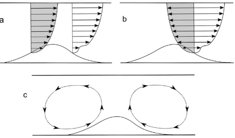
Sand waves are formed because of positive feedbacks between tidal currents and a sandy bed. Since a bed is never completely flat, these oscillating currents result in vertical recirculating cells, which transport sediment from the troughs to the crests.

2.3. Sand waves 11

Figure 2.4: Flow field upstream and downstream of a sand wave for flow in one direction (a), flow field on one side of a sand wave for flow in ebb and flood directions (b) and vertical recirculating cells (exaggerated) as a result of a tide averaged flow on both sides of a sand wave (c) (Choy, 2015)

2.3.3.

Migration

Following Besio et al. (2004) and Nemeth et al. (2002) they considered horizontal migration of sand waves due to asymmetries in the tidal flow. In Figure the circulations cells and the bed forms show stable pattern, when there is a disturbance in the tidal flow this results in an asym-metric profile of them both. The residual flow is responsible for the disturbance in the tidal flow, which result in sand wave migration, in the direction of the residual current.

The migration of the sand waves is very important in respect to the navigation channels. As can be seen in Figure 2.3 the sand waves are located near the navigation channels. When the sand waves migrate into the navigation channels, it is possible the channels are not deep enough to let ships pass. Rijkswaterstaat is responsible for the maintenance of the channels and has to guarantee a minimal depth. This is done by dredging the navigation channel throughout the year. A lot of pipe and cable lines lie in the seabed, like electricity, telephone, oil and gas lines. The diameter of the pipelines are between the 0.1 and 1.5 metres and are buried minimal 0.2 to maximal 2 metres in the seabed (Morelissen et al., 2003). Because there is migration of the sand waves and other bottom patterns, the cables and pipes can be exposed (Figure 2.5).

Chapter 3

Bathymetric data study

The first part of this study is to analyse bathymetric data. For the collection of bathymetric data vessels are used to survey the sea bed. The influence of the sandpits on current sand wave fields is analysed in this bathymetric data study. This chapter describes the analysis from the bathymetric data collection to results. First the studied location has to be determined and after that the bathymetric data is implemented in the method of Van Dijk et al. (2008) to get the sand wave characteristics. Following up, the migration rate of the sand wave fields are determined by linear regression.

3.1.

Collecting bathymetric data

The Hydrographic Service of the Royal Netherlands Navy is the government office which informs mariners about shipping channels, the seabed and underwater hazards such as obstructions like wrecks. In order to be able to inform them, the Hydrographic Service produces nautical charts and products, and issues Notices to Mariners. The nautical charts are based on bathymetric surveys which are done with two vessels of the Royal Netherlands Navy; HNLMS Luymes and HNLMS Snellius. Because the sea floor is changing with time, the bathymetric surveys should be carried out regularly. To survey the sea floor the vessels have to carry a lot of equipment. In the next paragraph 3.1.1, the sensors on the vessels will be explained.

3.1.1.

Collecting devices

The measuring equipments have to collaborate with each other to give a view on the sea floor. Figure 3.1 gives an overview of the di↵erent devices and explained briefly.

Singlebeam echo sounder: The singlebeam echo sounder measures the water depth directly

beneath the vessel. The hull-mounted transceiver transmits a high-frequency acoustic pulse in a beam directly downward into the water column. Acoustic energy is reflected o↵the sea floor beneath the vessel and received at the transceiver. The transceiver contains a transmitter, which controls pulse length and provides electrical power at a given frequency. To calculate the actual speed of sound through the water column the salinity, temperature and pressure need to be taken into account. This transmit-receive cycle repeats at a fast rate, in the order of milliseconds. On board the vessels, three single beams are present, each has its own frequency to detect di↵erent types of soil. The single beam is nowadays used as a control device for the multibeam echo sounder.

Multibeam echo sounder: A multibeam echo sounder is a device to determine the depth

of water and nature of the seabed. The multibeam transmits acoustic waves in a shape of a fan from directly beneath the vessel’s hull. The system measures and record the time it takes for the acoustic signal to travel from the transducer (transmitter) to the sea floor and back to the receiver. In this way, the multibeam transducer produces a “swath” of soundings for broad coverage of a survey area. The coverage of the sea floor depends on the depth of the water, typically two to four times the water depth.

Side Scan Sonar (SSS): The SSS emits pulses down toward the seafloor across a wide

3.1. Collecting bathymetric data 15

Magnetometer: The magnetometer is used to detect metal objects at the sea bottom, such

as pipelines, cables and part of wrecks. The magnetometer is towed approximately 250 metres behind the vessel, if this distance becomes less, the magnetometer will detect the vessel itself.

Moving Vessel Profiler: The Moving Vessel Profiler (MVP) is dropped into the water

ev-ery 15 minutes and will measure the speed of sound at various depths through the water column. The probe will measure temperature, speed of sound and pressure. The sound velocity through the water column will change, caused by changing temperatures, pressure and salinity of the water. The speeds of sound will be applied to the multibeam and singlebeam echo sounders to establish the correct depth values.

Global Navigation Satellite System (GNSS):GNSS is a satellite navigation system with

global coverage. Two GNSS systems are GPS (Global Positioning System) and GLONASS (Global’naya Navigatsionnaya Sputnikovaya Sistema). Without using a positioning system on board the surveys are not accurate.

Motion Reference Unit (MRU): The MRU is a heave, roll and pitch sensor to

compen-sate for the vertical and horizontal movements of the echo sounder’s transducer and positioning system’s antenna.

The systems on board of the vessels are much more complicated and extensive, which is not relevant in this research.

3.2.

Location of the bathymetric data study

The requirements of selecting data are:

. The surrounding of the sandpit

. Data has to be available over more years . The quality of the data has to be sufficient

3.2. Location of the bathymetric data study 17

(a) Maximal change in velocity by low tide includ-ing wind with respect to an undisturbed bottom

(b) Maximal change in velocity by high tide includ-ing wind with respect to an undisturbed bottom

(c) Absolute di↵erence in flow direction by low tide including wind

(d) Absolute di↵erence in flow direction by high tide including wind

Figure 3.2: Maximal changes and influence of the pits (Klein and van den Boomgaard, 2013)

Table 3.1 gives a summary about the bathymetric surveys of the three areas. Area A and B are based on three data sets, one set from 2004, which was the first official survey with the multibeam echo sounder. This set gave an impression of the sea bottom geometry, but a lot of adjustments were made, which makes it unsuitable for analysis. The data from 2008 is doubtful, not all the data was gathered by the Hydrographic vessels and a lot of unknown adjustments were made by another company. These surveys are also not suitable for data analysis. The survey time is 2 years, which is very long for such a dynamic area. For area A and B the only data which remains for analysis is from 2012, which is not enough. The 2008 dataset from the anchorage area is surveyed and adjusted by Rijkswaterstaat, this data is the most trustful data from the 2008 series. The described reasons conclude that only the anchorage area is taken into account. A disadvantage of the anchorage area is that it is not located in the influenced area following Klein and van den Boomgaard (2013), so the influences of the pits are less visible in the analysis.

Table 3.1: The bathymetric surveys of the area around the sandpit. The HY stands for a survey of the Hydrographic Service and the first two numbers are representing the year.

Area A Area B Anchor Area Notes

HY04156-157 HY04156-157 First multi beam survey

HY08111-9 HY08111-8 HY08111-1 9 and 8 unusable, 1 usable

HY12111 HY12111 Usable

HY11324-12105 Usable

587-13 Usable (RWS)

HY14105 Usable

3.3. Bathymetric data analysing 19

3.3.

Bathymetric data analysing

The data analysis consists of three parts: first gathering the data, secondly determine the wave length and crest- and trough positions and at last calculate the migration rate. In the next paragraphs the methods will be described briefly, not with a lot of details.

3.3.1.

Method description to analyse the data

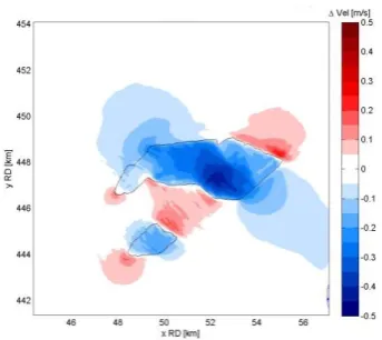
The data is gathered from the Hydrographic Service from the data sets as described in Section 3.2. The transect is located in the middle of the sand wave field and as much as possible selected perpendicular to the sand wave crests. The bathymetric data sets are all gathered at the same transect position in the anchorage area, which is represented with a black line in Figure 3.4. The height data is collected along the transect. A 1-D Fourier analysis is applied to the data, to separate sand waves from other bed forms by discarding wavelengths that do not correspond to the sand wave length spectrum. Following (Van Dijk et al., 2008) this sand wave length spectrum has to be chosen carefully.

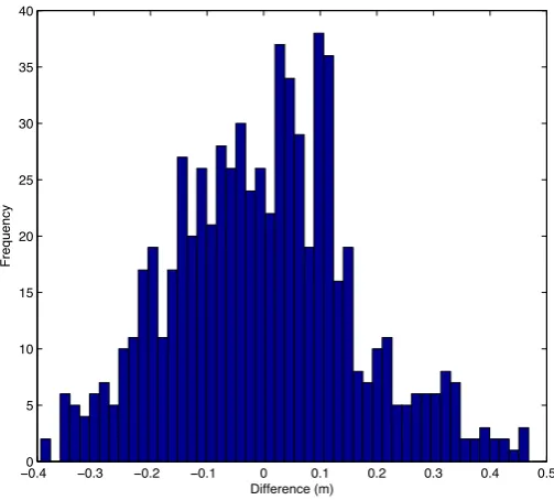
The model shows the wavelength from the di↵erent data in a graphic. From this point the minimum and maximum wavelength can be determined. Figure 3.5 shows a graphic of the data of 2011 from transect A, the power versus the wavelength. For Transect A a minimum wavelength of 63 metres and a maximum wavelength of 548 metres is chosen. The spectrum leads to smoothing the sea bed, which may result in a decreasing of the sand wave height. This is visible in Figure 3.6 were the di↵erence between the Fourier analyse and the Real Data visible is. In the bottom figure the absolute height-di↵erence is visible. The model gives also an error histogram, where the frequency of the di↵erence in height is visible. This histogram is also a check to determine the right wavelength (Figure 3.7). The smaller the maximal and minimal range and the higher the frequency o↵zero, the smaller the error is. After eliminating all the other bed forms, the crest and trough points are selected. The model (Van Dijk et al., 2008) calculates:

. The wavelength, which is defined as the length segment connecting two consecutive troughs

. The sand wave height, which is defined as the line perpendicular tot the base line segment, connected to the selected crest points

. The assymetry index, which is defined as the ratio between the length of the toss- and lee side of the sand wave

0 200 400 600 800 1000 1200 1400 1600 1800 0

0.05 0.1 0.15 0.2 0.25 0.3 0.35 0.4

Power

Wavelength (m)

3.3. Bathymetric data analysing 21

0 119 238 357 476 595 714 833 952 1071 1190 1309 1428 1547

−19 −18 −17 −16 −15 −14 −13 Distance (m)

Water depth (

−

m)

RD (Real Data) FA (Max. freq. 37) FA (Max. freq. 7)

0 200 400 600 800 1000 1200 1400 1600 1800

−2 −1 0 1 2 Distance (m) Amplitude (m)

FA(37) − FA(7) RD − FA(37)

Figure 3.6: The Fourier analysis versus the real data, Transect A year 2011.

−00.4 −0.3 −0.2 −0.1 0 0.1 0.2 0.3 0.4 0.5

5 10 15 20 25 30 35 40 Difference (m) Frequency

The model selects the crest and trough points, next you have to confirm them manually. It is important that all bathymetric data sets use the same crest and trough points, otherwise the data is compared with other sand waves. This is also the case with the inflection points, which are also selected manually and used to determine the gradient of the sand waves. Figure 3.8a represent the manually selected crest and trough points for Transect A of data the set 2011 and Figure 3.8b for the inflection points.

0 200 400 600 800 1000 1200

−2 −1.5 −1 −0.5 0 0.5 1 1.5 2 2.5 Amplitude (m) Distance (m) (a)

0 200 400 600 800 1000 1200

−2 −1.5 −1 −0.5 0 0.5 1 1.5 2 2.5 Amplitude (m) Distance (m) (b)

Figure 3.8: Selecting the crest and through points, a green circle is a selected- and red a deselected Crest/Through point.(a) Selecting the inflections points, a green circle is a selected- and red a deselected Crest/Through point.(b) Both are represent Transect A, year 2011

3.3. Bathymetric data analysing 23

To determine the uncertainty of the models a second transect is chosen, namely Transect B, which is also represented in Figure 3.4. This transect has a di↵erent angle and is situated on the edge of the sand wave field. Based on Figure 3.9 a minimum wavelength of 59 metres and a maximum wave length of 456 metres is chosen for Transect B. The calculated sand wave characteristics for each transect can be found in Appendix A.1.

0 200 400 600 800 1000 1200 1400 1600 1800 0

0.05 0.1 0.15 0.2 0.25 0.3 0.35 0.4

Power

Wavelength (m)

3.3.2.

Migration rates from bathymetric data

The wavelength, height and ratio between the lee and toss side has been calculated for each transect. The results for every sand wave of both transects can be found in Appendix A.2. With the sand wave characteristics the migration rate can be determined by linear regression. The crest migration rates of the transects over the years are displayed in Figure 3.10 and 3.11.

1 2 3 4 5 6 7 8 9 10

2 2.5 3 3.5 4 4.5 5 5.5 6 6.5 7

Sand wave number

Migration rate [m/year]

Overall Before After

Figure 3.10: The migration rate for the di↵erent sand waves on Transect A.

In Figure 3.10 it is visible that the migration rate over all the years has a range between 5.9 and 4 meters a year. In the before stage the migration rate fluctuated between 3.9 metres and 6.9 metres a year. The migration rate at the after stage for Transect A fluctuates between 5.8 and 2.6 metres. The maximal di↵erence is for both stages almost 3 metres, while this is larger than the calculated migration rate over all the years. Based on this numbers there is not a significantly di↵erence between the before- and after stage.

3.3. Bathymetric data analysing 25

A B C D E F G H I J K L M

2 2.5 3 3.5 4 4.5 5 5.5 6 6.5 7

Sand wave character

Migration rate [m/year]

Overall Before After

Figure 3.11: The migration rate for the di↵erent sand waves on Transect B.

The di↵erences between both transects are considerably, while the migration rates are calcu-lated for the same sand wave field. Both transects are illustrating that the place and orientation is very important to determine the migration. Selection of the a transect have a lot of uncertainty.

Because the migration of some sand waves are calculated by both transect, there is also a com-parison made between the corresponding sand waves. This is shown in Table 3.2.

Table 3.2: Migration rates in metres per year for both transects (A and B). For the ’Overall’, ’Before’ and ’After’ stage.

Sand wave Sand wave A. B. A. B. A. B.

number character Overall Overall Before Before After After

1 F 5.7 4.7 6.9 3.6 5.8 5.1

2 G 5.5 5 4 2.6 5.1 6.4

4 I 5.1 4.2 4.3 3.3 4.7 5.1

5 J 5 4.3 4.3 4 5.1 6.4

6 K 5.3 4.2 4.9 2.9 5.8 4.9

Chapter 4

Model set up

The used models are described in this chapter. How the models work, but also the needed input is described. First an overview is given from the taken steps.

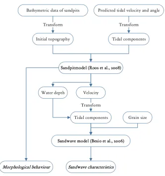
Figure 4.1 gives an overview over the used model applications and which input is needed.

The steps named briefly:

. First the bathymetric data is gathered from the sandpits. This data is used to generate the initial topography as input for the sandpit model.

. The predicted tidal velocity has to be transformed into several tidal components. How the transformation is done is described in subsection 4.1.2. After the transformation the values can be used as an input for the sandpit model.

. The sandpit model calculates the morphodynamic behaviour over the morphological times. The working of this model is briefly described in section 4.1.

. The output of the sandpit model is used as an input for the sand wave model. Before the output can be used it has to be transformed in the right formation by changing the velocity in tidal components.

. The grain size of the sediment is a new parameter and used as an input for the sand wave model.

. Eventually the output of both models together could determine the morphological behaviour of the sandpits and the sand wave characteristics in the surrounding area and in the sandpit.

Bathymetric data of sandpits

Transform

Initial topography

Predicted tidal velocity and angle

Transform

Tidal components

Sandpitmodel (Roos et al., 2008)

Velocity Water depth

Grain size Transform

Tidal components

Sandwave model (Besio et al., 2006)

Morphological behaviour Sandwave characteristics

4.1. Sandpit model 29

4.1.

Sandpit model

The sandpit model (Roos et al., 2008) is used to implement the current situation of the sandpits in the North Sea. The results show the morphodynamic e↵ect on morphological scale. The velocity results will be used as input for the sand wave model. A brief description about the model will be given, which is important to interpret the results.

4.1.1.

Description

The sandpit model is designed to investigate hydrodynamic e↵ects and morphodynamic impact of large-scale o↵shore sand extraction, with a focus on the pit geometry. With this model the long-term impact of large-scale sand extraction on the morphology and tidal flow of the seabed can be studied. This includes the sandpit as well as its surroundings.

The model is based on an idealised process-based model of sandbanks from Hulscher et al. (1993). The first step is to define the pit geometry of the bathymetric data, the orientation an-gle, the flow velocity and the mean water depth. The boundary conditions with a spatial domain have to be specified and should be much larger than the length of the pit. The depth-averaged hydrodynamic model uses two-dimensional shallow water equations, including Coriolis e↵ects and bottom friction. The basis equations are the conservation of momentum and mass and are expressed as:

g@⇠

@x+

@u

@t +u

@u

@x+v

@u

@y f v+

⌧bx

⇢D = 0 (4.1)

g@⇠

@y +

@v

@t +u

@v

@x+v

@v

@y f u+

⌧by

⇢D = 0 (4.2)

@D

@t +

@Du

@x +

@Dv

@y = 0 (4.3)

here isD=h+⇣ the total water depth,g the gravitational acceleration,uthe depth averaged horizontal flow velocity,vthe depth averaged vertical flow velocity,f the Coriolis parameter and ⌧b the bottom friction vector.

Some assumptions of the model are:

. The e↵ect of wind waves is neglected.

. The horizontal momentum dispersion is neglected.

. Chezy parameter is constant and uniform, i.e. the Chezy value is the same in- and outside the pit.

. Sediment, considered non-cohesive, is assumed to be transported as bed load mainly. . A threshold for sediment motion is neglected.

The model has a quasi-stationary approach and has two time scales: a ’fast’ hydrodynamic scale which refers to the tidal cycle and a ’slow’ morphological scale which refers to the bed changes. The time scales are widely spaced, so the bed changes within a tidal cycle can be neglected. With all this information the transport formula and the bed evolution can be given by:

*

q =↵|*u|3

*

u

|*u_|+

*

rh

!

,@h

@t =

*

r·D*qE (4.4)

This is including a downhill component. Here is ↵the proportionality coefficient in m 1_s2_, the dimensionless bed slope coefficient, *q = (qx, qy) the volumetric sediment flux in m2s 1,

u= (u, v) the flow velocity vector inx- and y-direction, hthe water depth,t the morphological time coordinate, r represents nabla-operator and the angle brackets denote averaging over a tidal cycle.

It is possible to calculate with di↵erent flow conditions, these conditions can be determined by the linear friction coefficient, phase lag and the several currents with the following Formula (4.5):

J(t) =M0+M2cos!t+M4cos(2!t ') (4.5)

It represents a unidirectional tide along thex-axis with a residual componentM0, a semi-diurnal lunar component of amplitudeM2 and its overtide (amplitudeM4, phase lag').

The model uses a spatial periodicity in x- and y- direction, to determine the spatial domain, the minimum wave number in the Fourier expansion has to be set. The relationship is explained by Lspace = _kmin2⇡ . In this case thekmin is 2.45⇥10 4. This corresponds with a spatial do-main of 25.6 kilometres. In simple words the model is constructed on a chessboard, on every box a pit is situated. It is important to choose a size of the box, that the pits on the board will not influence each other. Otherwise the results are not only influenced by one pit, but several.

The model output consists of seabed topography, time-dependent flow patterns and surface elevation. The results can indicate the position of the pit, its centre of mass and the area of morphodynamic influence. For this research it is useful to look into the pit, at the surroundings and at the location where the data research is done.

Some drawbacks to use the model for the specific Maasvlakte 2 case:

. The model uses an uniform depth outside the pits, which means that the assumption is a flat bottom. In the North Sea this is not the case. The little perturbation at the bottom are eventually flatten out by the long-term modelling, but an overall gradient at the seabed is therefore neglected.

. The model uses only one roughness value, while the grain size di↵ers, especially the di↵erence between the grain size in the pit and outside the pit.

4.1. Sandpit model 31

4.1.2.

Input

To give a realistic view on the results, the input for the model is important. The input is based on the tidal current and the geometry of the sandpits, which should have the shape of the realised sandpit for Maasvlakte 2.

Tides

The tidal flow is very important for the model, these tides cause the velocity and direction of the flow, which determines the displacement of the sediment. The tidal flow in the model is described with Equation 4.5. The Hydrographic Service of The Netherlands Navy also calculates the velocity of the flow caused by the sea. The calculation is determined by the observations from di↵erent tidal measurements, which are monitored the whole year. The flow velocity is based on hydrodynamic model simulations and the predicted velocities are published in the HP33 (Dienst der Hydrografie, 2013). The predicted velocities are calculated in the first fifth (from the seven) layers of the water column. This means that lower part of the column, situated at the sea bed, is not included in the prediction.

The program NL tides (The Netherlands Hydrographic Service, 2013) is a digital version of the HP33, which show the predicted velocity and direction of the flow with a maximum frequency of 5 minutes. A total spring neap cycle is gathered for each season. With the program t tide of Pawlowicz et al. (2002) this spring neap cycle signal can be divided, by means of a Fourier analysis, in a M2, M4 and M6- signal. Because the sandpit model deals with M0, M2 and M4, only these information is taken into account.

Because the di↵erences in season were not large, the season spring is chosen as initial condi-tion. The di↵erences in the season is described in Appendix B, where also a larger explanation of the used method is given. The t tide results of the related tidal ellipse is shown in Figure 4.2. The sand pit model, as it is implemented, can only handle (as seen in Eq. 4.5) a bi-directional M2-tide and a M4-tide with a phase di↵erence with respect to the M2- velocity. So M0 and both ellipses M2 and M4 must be projected on the major axis of the M2-ellipse. In this way a vector arises, Table 4.1 gives an overview of the values for the phase and amplitude of the tidal components.

Table 4.1: Velocity and phase on the major axis of the M2 tidal flow.

Velocity Phase

[m/s] [ ]

M0 0.053

M2 0.746 321

−0.5 −0.4 −0.3 −0.2 −0.1 0 0.1 0.2 0.3 0.4 0.5

−0.5

−0.4

−0.3

−0.2

−0.1

0 0.1 0.2 0.3 0.4 0.5

velocity in u direction

velocity in v direction

Spring M2 Spring M4 Spring residual flow major axis

Figure 4.2: The tidal spring tide, the residual is very small and almost invisible by the major axis.

In AppendixB the transformation from an ellipse to a major axis and the tidal flow versus the used flow in the model is shown. A translation in time is needed to eliminate the phase from Equation 4.6 and arrive at Equation 4.5.

The amplitudes stay the same, only the phase di↵erence (') will be 39 . Figure 4.3 illustrates the di↵erence between ˆJ(t) andJ(t). The signals are the same (inclusive the amplitude), only the starting time is di↵erent (phase).

Eventually the model calculates the velocities patterns on a fixed location. The translation for the output of the sandpit model into the used velocity for the sand wave model is described in Appendix B.

ˆ

J(t) =M0+M2cos(!t 'M2) +M4cos(2!t 'M4) with:

'= 2'M2+'M4

4.1. Sandpit model 33

0 1 2

−0.8 −0.6 −0.4 −0.2 0 0.2 0.4 0.6 0.8 1

π

Amplitude [m/s]

J(t) ˆ

J₍t₎

Figure 4.3: The tidal flow J(t) versus J(ˆt) on the M2 major axis with a period of the total spring neap cycle.

Sandpit

Figure 4.4: The di↵erence between the grids, also the place of the intersection is visible

As already stated in the model description (section 4.1.1), the seabed around the pit has to be flat. However, in reality the seabed is not uniform and has a slope. Figure 4.5 gives an overview with the di↵erent ranges in depth of the sea bottom around the pits. The non-uniform depth makes it difficult to put the pits into the model, so the little pit is ’cut’ out and shifted to the same surrounding depth as the biggest sandpit. In this way a small bit of data of the smallest sandpit has been lost, but not significantly.

Figure 4.5: The depth ranges given in colours

4.1. Sandpit model 35

4.2.

Sand wave model

The sand wave model Besio et al. (2006) is used to study the sand wave characteristics in the surrounding area of the modelled sandpit. The model is a linear stability-based model and based on the physical equations for conservation of motion, but assumes idealized and simplified conditions (Dodd et al., 2003). The model can be used to predict the initial formation of the sand waves, but is not able to predict the long-term formation processes. Therefore the input from the sandpit model is used, to still get insight of the changes on the long-term time scale. The model predicts the conditions leading to the appearance of both tidal sand waves and sand banks and determines their main geometrical characteristics. The model is based on the study of the stability of the flat seabed configuration. This is done by considering small seabed perturbations and providing linear analysis of their growth. The input is based on the velocity and water depth, which is generated from output of the sandpit model. Also the grain size is an important factor. These inputs are discussed in the following paragraphs.

4.2.1.

Input

The water depth is generated from the output of the sandpit model. The positions of the local depths are discussed in Chapter 5.

Velocity

The sandpit model calculates the flow velocity, as given in Equation B.1 and B.2. The output is given in real- and imationair- tidal components. This is due to complex bed amplitude, where the growth rate has a complex quantity. The imagitonary part of the growth rate is associated with migration. And has to be solved by time dependent Fourier components, where among other the velocity is included. A translation is needed to use the flow velocity as input for the sand wave model. This translation is described in Appendix B. Only the amplitude of the M2 velocity component is used in the sand wave model, because this is the dominant flow velocity.

Grain size

4.3. Output 37

4.3.

Output

The sand wave model calculates whether the circumstances are present to form sand waves and if so it calculates the preferred wavelength, growth rate and wave numbers in both x- and y -direction. With these outputs the response time of the sand wave can be calculated with the following formula (Cherlet et al., 2007):

Tr⇤=

(1 por)p d

rd⇤!

with:

d⇤= d h0

d = (!h0) 2 (⇢s/⇢ 1)gd

(4.7)

Where r is the dimensionless growth rate, ! the angular frequency of the tide in rad/s, Por the sediment porosity, d the grain size of the sediment in meters, ho the main water depth in meters, d⇤ _{the dimensionless grain size, d the mobility number,⇢s the sediment density and⇢} the water density both inkg/m3_{. The used parameters are shown in Table 4.2.}

Table 4.2: Parameters for the sand wave model.

d ⇢s ⇢ g por !

[m] [kg/m3_{] [kg/m}3_{] g[m/s}2_{] - [rad/s]}

Chapter 5

Results

In this chapter the results of the model study are shown. The first part describes the results of the evolution of sandpits over the years. These results are used as input for the sand wave model. Also those results are shown and a comparison is made for the sand wave characteristics with-and without the swith-andpits implemented. Finally the results are given from the swith-andpit model where the navigation channel is implemented. The model setup has already been explained in Chapter 4.

5.1.

Sandpit morphodynamic evolution

In Figure 5.1 the results of the evolution of the pits are shown for a period of 10, 30, 50, 100, 150 and 200 years. From the figures the following conclusions can be made: i) the pits will migrate in the direction of the dominant flow (the positivex-axis), ii) the pits become shallower, iii) the slopes of the pits will flatten out, iv) at the side of the large pit shallow areas will appear and v) the small pit will move to the large pit and finally merge into the large pit.

−5 −3 −1 1 3 5 y ( km )

10 years 30 years 50 years

−4 −2 0 2 4 6

−5 −3 −1 1 3 5

x(km)

y

(

km

)

100 years

−20 −15 −10 −5 0 5

−4 −2 0 2 4 6

x(km) 150 years

−20 −15 −10 −5 0 5

−4 −2 0 2 4 6

x(km) 200 years

−20 −15 −10 −5 0 5

Figure 5.1: The morphological behaviour of the pit over time

Migration of the sandpits

5.1. Sandpit morphodynamic evolution 41

−4 −2 0 2 4 6

−5

−4

−3

−2

−1 0 1 2 3 4 5

x [km]

y [km]

H

I

G

Figure 5.2: The location of the transects (G,H and I)

−4 −2 0 2 4 6 8

−20

−15

−10

−5 0 5

x (km)

height (m)

0 years 10 years 30 years 50 years 100 years

0 1 2 3 4 5 6 7 −20

−15 −10 −5 0 5

x (km)

height (m)

0 years 10 years 30 years 50 years 100 years

Figure 5.4: Transect H

−4 −3 −2 −1 0 1 2 3 4 5 6

−25

−20

−15

−10

−5 0 5

x (km)

height (m)

0 years 10 years 30 years 50 years 100 years

5.1. Sandpit morphodynamic evolution 43

0 50 100 150 200

0 0.5 1 1.5 2 2.5 3 3.5 4

Time [y]

Migration of deepest point of the transect [km] G large pit_{G small pit}

I large pit

Figure 5.6: The absolute migration of the pits from Transect G and I over time

0 20 40 60 80 100 120 140

0 0.1 0.2 0.3 0.4 0.5 0.6 0.7

Time [y]

Migration of deepest point of the transect [km] _{H large pit}

H small pit

The small pit migrates faster in the first 10 years than the larger pit. This is possible caused by higher flow velocity in the smaller pit, due to a lower water depth. Eventually the smaller and larger pit will migrate almost with the same distance. That the migration of Transect H is lower is caused by a di↵erent direction of the transect. This concludes that the deepest point of the pit not only move in the positivex-direction but also in they-direction.

Also the migration rate in m/year between the modelled years is given in Figure 5.8 and 5.9. These results show that the migration rate of the deepest point of the pit is not stable. The highest migration rate takes place in the first years, then the migration rate will decrease and finally becomes stable for some years. The migration rate of Transect I between 150 and 200 years is very high, the reason is of this is the large pit becomes more shallow and the deepest point is flatten out. This is visible in 5.5.

0 50 100 150 200

0 0.005 0.01 0.015 0.02 0.025 0.03 0.035

Time [y]

Migration rate of deepest point of the transect [km/y]

G large pit G small pit I large pit

5.1. Sandpit morphodynamic evolution 45

0 20 40 60 80 100 120 140

−2

0 2 4 6 8 10 12x 10

−3

Time [y]

Migration rate of deepest point of the transect [km/y]

H large pit H small pit

Figure 5.9: The migration rate of the pits from Transect H in m/year

Edges flatten out

Due to the larger flow velocity at the surroundings of the pits the sediment at the seabed become in motion and is transported into the pit. In the pit the flow velocity will decrease, the sediment will settle down and the pit becomes shallower, which is shown in Figure 5.10. In this figure

dh

d⌧ is given over the years. (⌧) stands for the morphological time, in other words dh d⌧ is the

−5

−3

−1 1 3 5

y

(

km

)

10 years 30 years 50 years

−4 −2 0 2 4 6

−5

−3

−1 1 3 5

x₍km₎

y

(

km

)

100 years

−0.3 −0.1 0.1 0.3

−4 −2 0 2 4 6

x₍km₎ 150 years

−0.3 −0.1 0.1 0.3

−4 −2 0 2 4 6

x₍km₎ 200 years

−0.3 −0.1 0.1 0.3

Figure 5.10: The dh

5.1. Sandpit morphodynamic evolution 47

Depth of the sandpits

Figure 5.11 shows a graphic for the di↵erent depths of the transect for the deepest depth for each modelled year. For all the pits and transects the depth is increasing, first fast and after a while slower. Take into account that this not the deepest depth of whole the pit, but only for the transect.

0 50 100 150 200

−25

−20

−15

−10

−5 0

Time [y]

Depth of deepest point of the transect [m]

G large pit G small pit H large pit H small pit I large pit

Figure 5.11: The maximal depth of the Transects G,H and I over time

5.2.

Sand wave characteristics

For the sand wave characteristics the initial situation at the surrounded area is calculated, this is done before the pit is implemented. In this way the influence of the pit is better visible. The initial conditions are the same conditions as used as input for the sandpit model. For the sand wave model a depth of 24 metres is used. Because the M2 is the dominant tidal velocity, a value of 0.7742 m/s, equal to the amplitude of M2, will be used in the calculations. The grain size is chosen uniform for all locations, namely 375µm. (Rijkswaterstaat, 2013).

This calculation gives the following results: a wavelength of 376 metres, a growth rate of 0.05 and a sand wave response time of 7.7 years. This response time corresponds with the most dynamic sand wave field in the Belgian Continental Shelf, the Westerhinder, following Cherlet et al. (2007).

5.2. Sand wave characteristics 49

To study the influence of the sand wave characteristics five locations are chosen. The locations are shown in Figure 3.2. Based on the most dynamic areas in combination with the sand wave fields at the west side of the pits, position 1 and 2 are chosen. The third location is situated in the anchorage area. Location four is the no-influence area described by Klein and van den Boomgaard (2013) and finally for the fifth location a position in the deeper part of the pit is chosen.

For each position the results of the sandpit model and the sand wave model will be discussed. In Appendix C tables can be found of the tidal amplitudes, depth, growth rate, wave length and response time for every location. In the next paragraphs only textual explanation is present and for each location a small table of the output for the initial condition, 10, 50 and 100 years.

Sand wave field 1 Through the years the residual velocity (M0=0.062) will increase with

a maximum of 14%, while the M2 velocity amplitude and depth stay, with a maximum deviation of 2%, almost the same. This corresponds with small changes over the years, which is visible in the sand wave characteristics. The sand wave lengths are around 377 metres, the growth rate 0.05 and the response time is 6.6 to 7.5 years, which is lower than the initial condition. In this period the orientation of the sand waves will change 2 to the South.

Table 5.1: The sand wave characteristics at the location ’Sand wave field 1’

⌧ ✓ M0 M2 M4 'Me 4 h0 r L

years [ ] [m/s] [m/s] [m/s] [ ] [m] [-] [m]

Initial 90 0.072 0.744 0.053 321 24.0 0.05 376

10 92 0.064 0.758 0.060 318 24.0 0.05 375

50 92 0.067 0.766 0.060 324 24.0 0.06 379

100 91 0.069 0.761 0.059 324 24.0 0.05 375

Sand wave field 2 Compared to sand wave field 1 this field has the same influence but the

residual velocity is higher (M0= 0.069 m/s ), with an increasing up to 9%. Furthermore not a lot of di↵erences appear between the two fields; the magnitude of the values are almost the same and the wave lengths of field 2 are approximately 372 metres. The response time of field 2 is higher, but still has the same magnitude; 6.9 to 8.8 years. The orientation of the sand waves changes 5 to the South, which will reduce to 2 South.

Table 5.2: The sand wave characteristics at the location ’Sand wave field 2’

⌧ ✓ M0 M2 M4 'M_e 4 h0 r L

years [ ] [m/s] [m/s] [m/s] [ ] [m] [-] [m]

Initial 90 0.072 0.744 0.053 321 24.0 0.05 376

10 95 0.070 0.725 0.053 321 23.8 0.04 369

50 94 0.072 0.743 0.054 321 23.7 0.05 373

Anchorage areaThe location of the anchorage area is further away from the sandpits than the sand wave fields, this could mean that the influence of the pits is lower. The lower e↵ect is visible in the residual flow, M2 amplitude and the depth, all are not changing significant. This causes also no changes in the wavelength of 375 metres and a growth rate of 0.05. The response time has the same magnitude as both sand wave fields, which means that the anchorage area behaves like a sand wave field. The response time is therefore steady and the sand waves will keep the same orientation as the original situation.

Table 5.3: The sand wave characteristics at the location ’Anchorage area’

⌧ ✓ M0 M2 M4 'M_e 4 h0 r L

years [ ] [m/s] [m/s] [m/s] [ ] [m] [-] [m]

Initial 90 0.072 0.744 0.053 321 24.0 0.05 376

10 90 0.072 0.743 0.053 321 23.8 0.05 376

50 90 0.072 0.743 0.053 321 23.7 0.05 376

100 90 0.072 0.744 0.053 321 23.5 0.05 376

Non-influenced area The non-influenced area has the same distance from the pits as the

anchorage area, it is expected that the influences here are not significant. However, in this area there are more fluctuations visible than in the anchorage area. Following Klein and van den Boomgaard (2013) this was not an influenced area and as shown in Figure 1.2 there were no sand waves presented. This means that in the area ‘new’ sand waves and more influences will occur than expected. The residual flow will decrease, while at the other locations it is increasing. The response time will grow and has the same magnitude as the sand wave fields, from 7.8 to 9 years. The sand waves will keep the same orientation as in the initial condition.

Table 5.4: The sand wave characteristics at the location ’Non-influenced area’

⌧ ✓ M0 M2 M4 'M_e 4 h0 r L

years [ ] [m/s] [m/s] [m/s] [ ] [m] [-] [m]

Initial 90 0.072 0.744 0.053 321 24.0 0.05 376

10 89 0.071 0.742 0.054 321 24.0 0.05 376

50 89 0.070 0.739 0.054 321 24.1 0.05 374

5.2. Sand wave characteristics 51

Maximum depth in pitThe largest depth in the pit has not a fixed position, it changes with

the migration of the pit. Thex- andy-position is given in the table from the largest depth in the pit over the years (Table 5.5). The residual flow and M2 amplitude is increasing, while the depth is decreasing. It is expected that a decreasing depth will cause an increase of the velocity. During a period of 200 years the depth of the pit will decrease with 10 metres, but still it will be 10 metres deeper than the surrounded area. At the beginning, compared to the other locations, the wavelength is large, but after 200 years the wavelength is the same as the other areas. The growth rate and the response time are significant smaller than the values of the sand wave fields. This means sand waves occur and grow slow, in other words on a large time scale. Compared to the original situation the orientation of the sand waves changes 15 South and will reduce to 2 South during the period of 200 years.

Table 5.5: The sand wave characteristics at the location ’Maximal depth in pit’

⌧ x y ✓ M0 M2 M4 'M_e 4 h0 r L

years [km] [km] [ ] [m/s] [m/s] [m/s] [ ] [m] [-] [m]

Initial 90 0.072 0.744 0.053 321 24.0 0.05 376

10 1.3 0.5 101 0.049 0.482 0.039 323 43.1 0.00 858

50 1.8 0.4 100 0.056 0.500 0.039 320 41.1 0.00 777

100 2.8 0 96 0.066 0.523 0.038 320 39.0 0.00 696

Besides the model only calculates the sand wave dynamics with the given sediment size. If there is, or will be, silt present in the pit, no sand waves will occur Borsje et al. (2009). Therefore, an analysis is performed in order to find out what the influence is from the grain size of the sediment. The known parameters are velocity and depth, but the grain size is a rough estimation. With a grain size smaller than 0.13 mm or bigger than 0.96 mm no sand waves will occur, so it is plausible with the current circumstances sand waves will arise (0.13 mm<grain size<0.96 mm).

Conclusion

The sand wave characteristics for the di↵erent position will not change significantly. Which means that the influence of the sandpits on the existing sand wave fields is not or a little present. So the present characterises and dynamics will hold on for years.

That the sand wave characteristics in the first years are more influenced, than after a longer time, is because the pit will flatten out and therefore the impact of the pit on the velocity is less present.

5.3.

Practical application

The question that can be asked is what happens to the navigation channels to enter Rotterdam mainport. Therefore the navigation channels are implemented in the model. Because the dredg-ing activities are not taken into account, the channel will migrate like a sandpit. Figure 5.13 shows the behaviour of the pits and the channel for the first fifty years. The morphological time is smaller than without the channel, because the interaction between the pit and the channel is then better visible.

−5 −3 −1 1 3 5 y ( km )

10 years 30 years 50 years

−4 −2 0 2 4 6

−5 −3 −1 1 3 5

x₍km₎

y

(

km

)

100 years

−20 −15 −10 −5 0 5

−4 −2 0 2 4 6

x₍km₎ 150 years

−20 −15 −10 −5 0 5

−4 −2 0 2 4 6

x₍km₎ 200 years

−20 −15 −10 −5 0 5

5.3. Practical application 53

In Figure 5.13 it is visible that the ridge between the biggest sandpit and the navigation chan-nels will vanish in time. Because the chanchan-nels behave like a sandpit it will also migrate in the dominant flow direction, while in reality the positions are fixed caused by dredging activities. Because of the fixed positions the largest sandpit will reach the navigation channels sooner than the results show.

Figure 5.14 and 5.15 shows the transect of G and I, which are also taken in section 5.1. Here the di↵erence is shown of the sandpit and the navigation over a period of 50 years. In the first period of thirty years the largest decrease of the ridge, between the channel and pit, will occur. In the second period, after thirty years, the ridge will decrease in a lower rate and finally it will vanish. It is also visible that the slopes will flatten out and the pit becomes shallower. However, the navigation channel becomes deeper because of the connection between the pit and channel, and it will start behaving like a pit. This means that the merged pit will migrate in the flow direction and the bottom will become flattened.

−6 −4 −2 0 2 4 6

−20

−15

−10

−5 0 5

x (km)

height (m)

0 years 5 years 10 years 30 years 50 years

−6 −4 −2 0 2 4 6

−20

−15

−10

−5 0 5

x (km)

height (m)

0 years 5 years 10 years 30 years 50 years

Figure 5.15: Transect I, including the navigation channel

The deepest point of the transect is followed to determine the migration inx-direction. This is done for both transects and illustrated in Figure 5.6, the migration rate is illustrated in Figure 5.17.

In the first couple of years the pits migrate faster, but after those years the migration is almost stable. The increasing of transect I is due to the merging of the pit with the channel. By this merging the deepest point is included with the channel and therefore the deepest point is harder to follow, which conclude in a larger migration rate, which is not comparable with the other years.

The ridge between the large pit and the navigation channel vanish in time. In transect G the edge will eroded for the first 30 years and will totally be connected with the large pit. In transect I the edge needs a smaller time to vanish, namely 10 years. Over the years the edge become smaller and the flow need less e↵ort to reduce the edge, therefore the erosion of the edge becomes higher over the years.