iii
Abstract
Mobile robot navigation in an unknown environment is an important issue in autonomous robotics. Current approaches to solve the navigation problem, such as roadmap, cell decom-position and potential field, assume complete knowledge about the navigation environment. However, complete knowledge about the environment can be hardly obtained in practical ap-plications where obstacles locations and surface friction properties are unknown. On the other hand, navigation in an unknown environment can be phrased as a reinforcement learning (RL) problem, because it is only possible to discover the optimal navigation plan through trial-and-error interaction with the environment. The goal of this project is to control a skid-steering mobile robot to navigate in an unknown environment with obstacles and a slippery floor using reinforcement learning techniques. The main task studied is the navigation to a goal location in the shortest time while avoiding obstacles and overcoming the skidding effects.
The standard (model-free) Q-learning algorithm is widely used to discover optimal trajecto-ries in unknown navigation environments. However, it converges to these trajectotrajecto-ries with undesirably-slow rates. The Dyan-Q approach extends the Q-learning with online-constructed models about the environment properties (obstacles, slippage, etc.) resulting in a model-based Q-learning platform. In this thesis, we examine using a multinomial probabilistic model to de-scribe the state transition probabilities of the system dynamics. Moreover, two ideas to improve the learning performance of the Dyna-Q approach are suggested. The first is to prioritize the simulated learning experiences to be around the shortest discovered navigation trajectories between the initial and the target states. The second is to learn a parametric kinematic model for the robot motion that can be used to simulate the motion characteristics of the robot in unvisited locations.
It was shown that utilizing the models to simulate learning experiences makes the robot more robust to stochastic effects caused by skidding. The experimental results proved that the model-based RL algorithms converge faster to sub-optimal policies with higher success rates than the model-free Q-learning. Therefore, model-based algorithms have a better long-term performance in terms of less divergences from the discovered sub-optimal trajectories.
v
Contents
1 Introduction 1
1.1 Context . . . 1
1.2 Reinforcement learning . . . 1
1.3 Problem statement . . . 2
1.4 Literature review . . . 3
1.5 Project aims and objectives . . . 8
2 Background 10 2.1 Q-learning algorithm . . . 10
2.2 Dyna-Q algorithm . . . 12
2.3 Prioritized Sweeping . . . 14
2.4 Multinomial probabilistic models . . . 14
2.5 Skid-Steering-Mobile-Robots kinematic model . . . 15
2.6 Multi-output Bayesian regression . . . 18
3 Problem Analysis 21 3.1 System representation . . . 21
3.2 Q-learning parameters selection . . . 25
3.3 Dyna-Q-based navigation . . . 28
3.4 Motion analysis of Skid-Steering-Mobile-Robots . . . 30
4 Learning Algorithms Design 33 4.1 Dyna-Q platform design . . . 33
4.2 Learning SSMRs kinematic model . . . 40
4.3 Smart planning . . . 42
5 Experimental Design 44 5.1 Experiments in simulation . . . 45
5.2 Experiments in real-time . . . 49
6 Results 55 6.1 Simulation results . . . 55
6.2 Real-time experiments results (Slippery surface) . . . 65
6.3 Real-time experiments results (Rough surface) . . . 70
6.4 Discussion . . . 73
6.5 Reflection . . . 75
7 Conclusion 76
7.1 Future research . . . 77
A Appendix 78
A.1 Simulation codes . . . 78 A.2 Real-time codes . . . 91
Figure 1.2:Reinforcement learning decision making diagram for robots control.
The most common-used reinforcement learning algorithm in the literature to solve au-tonomous navigation is Q-learning [11]. The Q-learning optimal value function is defined as
Q∗(s,a)=E[R(s,a)+γmaxa0Q∗(s0,a0)] (1.1) This represents the expected value of the reward for taking actiona from states, ending in states0, and acting optimally from then on. The parameterγis known as the discount factor, and measures how much attention is paid to future rewards. Once we have the optimal Q-function for each state-action pairQ∗(s,a), it is easy to deduce the optimal policy,π∗(s), by simply selecting the action with the largest state-action pair value,
π∗(s)=ar g maxaQ(s,a) (1.2)
If the system is fully described by a set of finite states, the Q-function is typically stored in a ta-ble, indexed by the state-action pair. It is initialized by arbitrary values and iteratively updated to approximate the optimal Q-function based on the observation of the world. Every time that the robot takes an action, an experience tuble, (st,at,rt+1,st+1), is generated. The Q-function table for statesand actionais then updated as follows
Q(st,at)←(1−α)Q(st,at)+α(rt+1+γmaxa0Q∗(s0,a0)) (1.3) Under some reasonable conditions [26], this is guaranteed to converge to the optimal Q-function,Q∗(s,a). Q-learning is known aso f f −pol i c y RL algorithm. This means that the distribution from which the training samples are generated has no effect on the policy learned. 1.3 Problem statement
This research project aims to develop a RL-based navigation system to enhance the naviga-tion capabilities of skid-steering-mobile robots (SSMRs). These capabilities are quantified by the robot ability to discover navigation trajectories to move to a target location in mini-mum time avoiding obstacles and slippery areas. This will be achieved by overcoming the main challenges that are usually faced when formalizing a robotic navigation problem as a reinforcement-learning problem, namely [12]:
CHAPTER 1. INTRODUCTION 3
with m levels will result inmn different unique states. This exponential growth in the number of states leads to very slow convergence rates of the RL algorithm. It is possi-ble to discretize the 2D space of the motion to obtain a grid world representation of the map. However, in case of SSMRs with non-holonomic constraints, it is not possible to simply move in the lateral directions. Therefore, the action space is usually discretized with four actions (move-forward, move-backward, turn-left, and turn-right). These ac-tions are orientation-dependant necessitating including the robot orientation as a state [3]. Including the orientation as an internal state increases the dimension of the system so that the expected convergence time increases significantly.
• Curse of real-world samples:learning from interaction with the real environment is ex-pensive in terms of time, human supervision and finance as explained in [12]. It is es-sential to create efficient RL algorithms that can learn from a small number of trials with the physical environment instead of limiting the memory consumption or the computa-tional complexity.
• Curse of under-modelling and model uncertainty:One way to decrease the need to real-world interaction is to depend on accurate simulation models. However, small model er-rors due to under-modelling may cause the behaviour of the simulated robot to diverge from the real-world system. In SSMRs, sliding is an inherent motion property resulting in high levels of stochasticity in the robot model. Such property results in difficulties in ac-curately modelling the navigation environment due to the nonlinear stochastic slippage properties.
• Curse of goal specification: The goal of RL algorithms is to maximize the accumulated long-term reward. Although specifying the reward is simpler than detailing the behaviour itself, in practice, it is challenging to define a good reward function for the robot task. Since traditional binary rewards used in classical RL algorithms barely succeeds in prac-tical robotic applications, a reward can be fully specified in terms of features of the space in which the RL algorithm operates, a problem which is known asreward shaping. 1.4 Literature review
This section presents how the reinforcement learning paradigm has been combined in naviga-tion systems in the previous research. Based on the analysis of the previous research, the aims and the objectives of this research projects will be motivated.
1.4.1 State space representations
The representation of system states determines the dimensional properties of the system which have huge impacts on the speed of convergence of the RL algorithm. In [3], the pose states of the mobile robot [x,y,θ] were discretized with 15 quantization levels each. This results in a total system with 13500 state-action pairs. The experiment carried out took 15000 iterations for the algorithm to converge to the optimal policy given that the work-space dimensions are 1x1.2m. This relatively slow convergence rate has motivated representing continuous state spaces. This is achieved by extending the traditional Q-learning algorithm by a state-value approximation function. In the traditional Q-learning, the value of each state-action pair is tabularly repre-sented. However, value function approximators aim to learn a parametric function that can map each state-action pair to its optimal value. There are several possible representations for these parametric functions. In [17],[34],[30] where intensive sensor data are processed, the fol-lowing neural networks structures were utilized as value function approximators:
• Continuous state-space clustering: this approach has been presented in [17] to solve the structure credit assignment problem in the representation of the navigation environ-ment. This problem states that if the state space is highly discretized, the same credit
CHAPTER 1. INTRODUCTION 7
have noted the method by Environment Exploration Method (EEM). The navigation system has two basic modules: avoidance behaviour and goal-seeking behaviour. The avoidance be-haviour and the goal-seeking bebe-haviour are fuzzy engines that map the sensor readings to a fuzzy output which is the optimal action. The fuzzy rules are built using reinforcement learn-ing rather than supervised learnlearn-ing which requires less evaluation data.
In [35], they propose a navigator which consists of three components: obstacle avoidance, move-to-goal and a fuzzy behaviour supervisor. The obstacle avoidance components receives sensory data that are fuzzified then the rules are learned through RL. After constructing fuzzy rules, the decisions are made to generate the output actions. The same principle applies for the move-to-goal component. The fuzzy behaviour supervisor module receives the output of the other two components and generates an appropriate action. The result of the algorithm showed that this method produced higher performance and did not suffer from local minima. However, both methods are applicable only to static environments and cannot be utilized for dynamic ones.
An other hybrid approach is presented in [10]. This approach introduces an enhanced dynamic self-generated fuzzy Q-learning approach (EDSGFQL) for automatically-generated fuzzy infer-ence systems (FISs). The structure identification and the parameter estimations for the FISs are obtained using reinforcement learning. The Q-learning is used to cluster the input space to generate the FISs. Also, RL is used to adjust and omit fuzzy rules dynamically. EDSGFQL was used for a navigation task for a Khepera mobile robot. The simulations showed that the robot has succeeded in wall following and obstacles avoidance tasks for static environments. Another hybrid learning method that uses a fuzzy inference system structured based on the generalized dynamic fuzzy neural network algorithm was proposed by [9]. Supervised learning is applied for the neuro-fuzzy controller and a reinforcement-learning actor-critic method is used so that the system can re-adapt to a new environment without human interventions. The reinforcement learning is used to tune the parameters of the fuzzy rules. The simulations have proven the system ability to solve the obstacles avoidance problem in a static environment. Neural Q-leaning
As presented in the previous subsection, representing a continuous state space requires mod-ifying the standard Q-learning algorithm to include a value function approximator. In the context of autonomous navigation, neural networks have been used as efficient function ap-proximators. There are three neural network structures that have been used with Q-learning to achieve autonomous navigation which are presented in 1.4.1. The first method (state-space clustering) presented in [17] has a better convergence rate than the regular neural Q-learning method. In this approach, discrete Q-learning is used in stead of continuous Q-learning. The learning is based on clustering input data into similar and dissimilar groups. The method uses a discrete representation for the action space. The clustering algorithm performs faster than other neural Q-learning methods but it is only applicable to static environments [11].
The probabilistic roadmap method (PRM) has been combined with the Q-learning to im-plement a hybrid approach for the robot navigation in [21]. The PRM method is based on connecting the start location of the robot to the target location by drawing random nodes in an assumed obstacles-free space. The Q-learning is used when an obstacle blocks a pre-planned trajectory to determine the best action to be taken to avoid the obstacle. The performance of the method is degraded for dynamic navigation environments.
1.4.3 Reward shaping
The are several ways to shape the reward function to solve the navigation problem. These ways are listed below:
• Binary reward: This is a very simple strategy. It gives 1 reward on reaching the goal and zero otherwise. This strategy is commonly-used in classical reinforcement learn-ing problems that do not include a dynamical behaviour. Adoptlearn-ing this method makes the convergence rate very slow specially in highly-dimensional state spaces where the probability of finding the goal is significantly small [26].
• Sparse reward:It is similar to the binary reward. In addition, it adds negative reward on hitting the obstacles and zero otherwise. This approach to shape the reward function has been used intensively in the literature ([25], [26] and [3]).
• Potential-based reward: this idea has been introduced in [20]. It aims to find a trans-formation to the sparse reward function that incorporates knowledge about the naviga-tion environment in the design of the reward funcnaviga-tion. The approach assigns a potential valueφ(s) to each cell in the navigation grid. This potential is determined based on the distance between the cell and the goal and the distance between the cell and known ob-stacles. The transformation applied to the sparse reward will beR0=R+Fwhere
F(s,a,s0)=γφ(s0)−φ(s) (1.12) 1.4.4 Conclusion
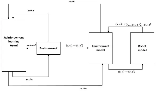
From the previous review it can be seen that there is a trend among the researchers to adopt the continuous neural Q-learning to solve the navigation problem. On the other hand, they did not address the potentials of including environment models together with the reinforcement learning to accelerate the learning process. This approach is known asmodel-based reinforce-ment learningorindirect reinforcement learning. The idea has been introduced in [4], [27] and [23] where several model-based Q-learning algorithms like dyna-Q and prioritized-sweeping were elaborated. Although they provide great potentials in speeding up the convergence rate of the Q-learing, they have not been used intensively in the RL-based autonomous navigation. Similarly, models for robot motions are not commonly utilized to plan motion trajectories to-gether with the reinforcement learning. Moreover, the problem of slippery surfaces and sliding motion of SSMRs are not addressed in the literature. These reasons motivate directing the re-search of this project to the area of integrating models with standard Q-learning. We suggest learning several models online (an environment model, a robot model and a slippage model). These models are used to extend the standard Q-learning algorithm to achieve (sub)optimal motion trajectories.
1.5 Project aims and objectives
The common trend in the current research is to combine standard Q-learning algorithm with neural networks to accelerate the learning process (Neural Q-leaning). On the other hand, the model-based reinforcement learning is proven to accelerate the convergence rate more than the standard Q-learning [4]. The aim of this project is to explore the potentials of the model-based reinforcement leaning for autonomous navigation tasks in unknown stochastic environ-ments. This is obtained by modifying the standard Q-learning algorithm by extending it with online learned models of the robot motion and the navigation environment (obstacles loca-tions and slippage properties). The aim of the project can be accomplished through exploring the following research objectives:
• How to model the transition of the robot states in the environment stochastically? • How to model the motion of the SSMR robot to integrate it with the Q-learning algorithm? • What is the effect of discretization level of the action and the state spaces on the learning
CHAPTER 1. INTRODUCTION 9
• What is the effect of including models with the standard Q-learning on the performance of the reinforcement-learning system?
Motivated solutions are validation by designing a RL-based navigation system for a small SSMR so that it can explore optimal trajectories to given targets in an unknown environments. This report shows the research work aimed to achieve these research objectives and is orga-nized as follows:
Chapter 2summarizes the theories involved in the design of the RL-based navigation systems. It elaborates more on the standard Q-learning algorithm and how to modify it to implement a model-based reinforcement learning through the Dyna-Q algorithm. Then, it introduces multinomial probabilistic models which will be used to model the transition of discrete system states based on data gathered from the environment. Finally, it introduces the kinematic model of SSMR and Bayesian ridge regression algorithm used to estimate the SSMR kinematic model using the data gathered from the robot and the environment.
Chapter 3shows how the navigation problem can be formulated as a reinforcement learning problem to be solved using a model-based Q-learning algorithm. Firstly, it explains require-ments on the system representation necessary to use the Q-learning algorithm. Then, it dis-cusses selecting the parameters of the Q-learning algorithm in the context of the autonomous navigation. After that, it analyzes the nature of motion of Skid-Steering-Mobile-Robots elabo-rating the requirements needed to model their motion. Finally, it shows the set-up built to run the real experiments and the limitations it introduces to the system performance.
Chapter 4proposes a design structure of a reinforcement-learning-based navigation system. The learning system is designed based on the Dyna-Q platform modified by creating a multi-nomial probabilistic model to describe the dynamics. The algorithm is enhanced by creating an online-structured Bayesian regression model to learn the kinematic model of the mobile robot. Finally, the architecture of the software used to run the set-up in real-time is presented.
Chapter 5provides a detailed analysis of the obtained results of the simulation and the real-time experiments.
2 Background
2.1 Q-learning algorithm
2.1.1 Finite Markov decision process
The solution of reinforcement learning problem is framed by modelling the control process as a finite Markov decision process (MDP) [28]. In a MDP, the controller is called theagent and everything outside the agent is called theenvironment. The agent at stateSt can interact with
the environment (figure 2.1) by applying an actionAtand the consequence of this interaction
[image:16.595.156.415.257.349.2]is receiving a numerical rewardRt+1(a scalar value needed to be maximized by the agent over time) and the agent moves to a new stateSt+1.
Figure 2.1:The agent-environment interaction in a Markov decision process [28].
In a finite MPD, there are two random variablesRandSwith a well-defined discrete probability distribution that depends only on the current statesand the applied actiona. So for all next states0∈S,r∈Randa∈A(s) it applies:
p(s0,r|s,a)=P r[St=s0,Rt=r|St−1=s,At−1=a] (2.1)
X
s0∈S X
r∈R
p(s0,r|s,a)=1 (2.2)
The probabilitiesp completely characterize the environment’s dynamics. If it is sufficient to know the current statest and the current action at to determine the probability of the next
statest+1and the next rewardrt+1then the system is said to have the Markov property. The expected rewards for state-action-next state pairs as a three-argument functionr:S×A× S→ ℜ,
r(s,a,s0)=E[Rt|St−1=s,At−1=a,St=s0] (2.3)
The agent’s goal is to maximize the total amount of this expected reward received from the environment. This means maximizing not the immediate reward, but the cumulative reward in the long run. If the sequence of rewards received after time stept denotedRt+1,Rt+2,Rt+3, ...,
then maximizing the value of this sequence is denoted by maximizing theexptected return, where the returnGt:
Gt=Rt+1+Rt+2+Rt+3+....+RT (2.4)
whereTis a final time step. If the task representing the agent interaction with the environment can be naturally broken into sequences that end with a specific terminal stateS+, then this task is called anepisodic task. In episodic tasks, the agent’s state is reset to a starting state after reaching the terminal state. The time of terminationTis a random variable that normally varies between episodes. It is also possible to discount future rewards to be maximized by introducing the discount rate parameterγwhere 0≤γ≤1. Thus, the goal is to maximize the discounted return:
Gt=Rt+1+γRt+2+γ2Rt+3+....= ∞ X
k=0
CHAPTER 2. BACKGROUND 11
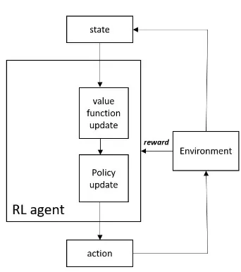
2.1.2 Policies and value functions
Reinforcement learning algorithms involve estimating value functions. They are functions of states (or of state-action pairs) that estimate how good for the agent to be in that state in terms of maximizing the future reward. Since the rewards to be received in the future depends on the actions taken, value functions for system states depend on the strategy adopted to select actions which are calledpolicies. A policyπdefines a probability distribution of selecting an actionaat each states(π(a|s)) for eacha∈A(s) ands∈S. Thevalue functionof a statesunder a policyπ, is the expected return starting fromsfollowingπ:
vπ(s)=Eπ[Gt|St=s]=Eπ[
∞ X
k=0
γkRt+k+1|St=s] (2.6)
Similarly, the action-value function of actionain statesunder policyπis defined:
qπ(s,a)=Eπ[Gt|St=s,At=a]=Eπ[
∞ X
k=0
γkRt+k+1|St=s,At=a] (2.7)
The reinforcement learning problem is solved by finding the policy that maximizes the reward over the long run. A policyπ0is said to be better a policyπ(π0>π) if and only ifvπ0(s)>vπ(s) for alls∈S. There is always at least one policy that is better than or equal other policies which is theoptimal policy. Optimal policies share the same optimal action-value function, denoted byq∗:
q∗(s,a)=max|πqπ(s,a) (2.8)
This optimal action-value function gives the expected return of taking an actiona in state s
following the optimal policy:
q∗(s,a)=E[Rt+1+γv∗(St+1)|St=s,At=a] (2.9)
2.1.3 Off-policy Q-learning
The Bellman optimality equation states that the value of a state under an optimal policy must equal the expected return of the best action at that state:
v∗(s)=max|a
X
s0,r
p(s0,r|s,a)[r+γv∗(s0)] (2.10)
This last equation represents the Bellman optimality equation forv∗. The Bellman optimality equation forq∗is
q∗(s,a)=max|aX s0,r
p(s0,r|s,a)[r+γmax|a0q∗(s0,a0)] (2.11)
For finite MDPs, the Bellman optimality equation forvπhas a unique solution independent of
the policy. The Bellman optimality equations for an n states system is a system of n equations in n unknowns. If the dynamicspof the environment are known, then it is possible to solve for
v∗by solving systems of non-linear equations and consequently solving a related set of equa-tions forq∗. If the dynamics of the environment are unknown, it is still possible to estimate the optimal action value functionsq∗through the experience by interacting with the environment and updating a numerical back-up equation for each state-action pair valueQ(s,a).
Q-learning algorithm (figure 2.2) is a powerful tool for estimating the optimal action value func-tionsq∗of a stochastic Markovian system with unknown dynamics. It uses the following back-up back-updating rule:
Q(St,At)←Q(St,At)+α[Rt+1+γmax|aQ(St+1,a)−Q(St,At)] (2.12)
Where 0<α≤1 parameter is called thelearning rate. Under the usual stochastic approxima-tion condiapproxima-tions, Q-learning algorithm converges with probability 1 toq∗if all the state-action pairs are visited and updated. Thus, the policy to be followed during the exploration phase of the environment is not the learned optimal policy (greedy) policy. In stead, actions are selected randomly with a probability²at each state to enhance exploring new state-action pairs. This exploration policy is called the²−g r eed ypolicy. Since the learned policy through the back-up updating ruleπ∗ is different from the policy followed during the learning process, Q-learned is called an off-policy reinforcement learning algorithm. In this case, the learned action value function Q, directly approximateq∗independent of the policy being followed.
Figure 2.2:Q-learning algorithm for approximatingq∗[28].
2.2 Dyna-Q algorithm
Q-learning algorithm is amodel-freereinforcement learning algorithm since it depends only on learning to update action value functions for each state-action pair. On the other hand,
model-basedreinforcement learning algorithms depend on planning using a model of the en-vironment structured online during learning [28]. A model of the enen-vironment allows the agent to make predictions about the next states and the next rewards. If the system is stochastic, en-vironment models produce a description of all possibilities with their probabilities leading to
probabilistic distribution models.
CHAPTER 2. BACKGROUND 13
Figure 2.3:The general Dyna-Q architecture [28].
If planning is done online while interacting with the environment, collected data representing state transitions are used to modify the model and consequently affect the planning. Dyna-Q architecture, shown in figure 2.3, is a platform proposed in [27] that integrates model-learning, planning and value functions updating. After each interaction with the environment, the ex-perience (St,At→Rt+1,St+1) is used for the planning update (figure 2.3). Moreover, it is stored
in a look-up table that maps each (St,At) to equivalent (Rt+1,St+1). This model learning based
assumes that the model is deterministic. During planning, the Q-planning algorithm randomly samples only from state-action pairs that have been experienced before and stored in the ta-ble. The data stored in the table-based model are used to simulate hypothetical experiences that can directly update the Q-values of state-action pairs just as if they really happened. The agent performs N hypothetical experiences after each real-world interaction with the environ-ment. The same back-up update rule is used both for learning from the real experience and for planning from simulated experiences.
Figure 2.4:The tabular Dyna-Q algorithm [28].
Figure 2.4 shows a pseudo-code of the general Dyna-Q algorithm that assumes a deterministic environment. Integrating planning with learning accelerates the convergence to the optimal
q∗significantly. Because any change in the q-value of a state-action pair is going to propagate to values of other pairs through hypothetical experiences. On the other hand, when a new information is gained, the model is updated and the planning will decide different ways of behaving based on the updated model.
2.3 Prioritized Sweeping
[image:20.595.94.475.236.451.2]The Dyna-Q algorithm presented in the previous chapter selects state-action pairs to simulate hypothetical experiences uniformly from the stored experience. The hypothetical experiences can be more efficient if the simulated updates are focused on particular state-action pairs. The prioritized sweeping algorithms focuses on state-action pairs whose values have changed re-cently. If the values of these pairs have changed, then the values of the predecessor states may change accordingly. Then, actions leading into them needed to be updated, and then their pre-decessor states may have changed. Thus, the algorithm works backward from arbitrary states that have changed their values, either performing updates or ending the propagation. This idea is calledbackward focusingof planning computations.
Figure 2.5:The tabular prioritized sweeping algorithm [28].
It is convenient to prioritize the updates based on the change of the state-action pairs values and perform them in order of priority. The planning algorithm performs this idea is called
prioritized sweeping. The state-action pairs are stored in a priority queue being updated based on the change of each state-action pair value prioritized by the amount of the change. When the top of the queue is updated, the effect on each predecessor pair is computed. If the effect generates a pair value greater than a threshold, the pair is inserted in the queue with a new priority. In this way, the effects of changes are efficiently propagated until stillness. The full algorithm is explained in figure 2.5.
2.4 Multinomial probabilistic models
The general Dyna-Q algorithm presented in the previous section assumes a deterministic envi-ronment. However, in the context of autonomous navigation for SSMRs, sliding is an inherent system property that leads to stochastic dynamics. Thus, the learned model should be proba-bilistic. The basic idea to learn a probabilistic model is that not predicting a deterministic next state and a deterministic reward, but a probability distribution over next states and next re-wards [27]. For discrete finite MDPs, it is possible to represent the state transition probabilities
p(s0,r|s,a) using multinomial distributions [14].
CHAPTER 2. BACKGROUND 15
the remaining elements are 0. Such vectors satisfyPK
k=1xk=1. If the probability ofxk=1 is denoted by the parameterµk, then the distribution ofx:
p(x|µ)= K
Y
k=1
µxk
k (2.13)
whereµ=(µ1, ..,µK)T such thatµk≥0 andPkµk=1. Now consider a data setDofN
indepen-dent observationsx1, ..,xN. The corresponding likelihood function takes the form:
p(D|µ)= N Y n=1 K Y k=1
µxnk
k = K Y k=1 µ( P
nxnk)
k =
K
Y
k=1
µmk
k (2.14)
mk=Pnxnkrepresents the number of observations ofxk=1. Given the data setDit is required
to solve forµ. This solution is achieved by findingµthat maximizes the likelihood function. Maximizing the likelihood is achieved by maximizing its logarithmic functionl n[p(D|µ)] ac-counting for the constraintP
kµk=1. This can be achieved by using a Lagrangian multiplierλ: K
X
k=1
mkl n(µk)+λ K
X
k=1
µk−1 (2.15)
By setting the derivative of the previous equation with respect toµkto zero, the solution forµk
is:
µk= −mk/λ (2.16)
To solve for the Lagrangian multiplierλ,(2.16) is substituted into the constraintP
kµk=1. Thus,
the maximization of the likelihood is given in the form:
µkM L=mk
N (2.17)
which is the fraction of theN observations whosexk =1. Themultinomial distributionis a
joint distribution of the quantitiesm1, ...,mk given the parameterµon the total number of N
observations. It takes the form:
Mul t(m1, ..,mK|µ,N)=
N!
m1!m2!..mK! K
Y
k=1
µmk
k (2.18)
The normalization coefficient is the number of ways to partitionN objects intoK groups of sizem1, ..,mK. These variablesmkare subject to the constraint:
K
X
k=1
mk=N (2.19)
2.5 Skid-Steering-Mobile-Robots kinematic model
The previous section shows how it is possible to build probabilistic models for the next states and rewards for each state action pair (s,a) given the experience data set (D=(s10,r1)..(s0N,rN)).
This means that it is only possible to simulate hypothetical experiences for already-visited state-action pairs (s,a). If it is required to predict probability distributions for the next states and rewards for action-action pairs that have not been visited before, an accurate model for the robot motion must be developed. This model is also necessary for simulating the designed reinforcement learning algorithms before validating them in real-time.
In [13], a kinematic model for SSMRs is presented. This kinematic model can be developed by analyzing the robot free body diagram shown in figure 5.2 .
Figure 2.6:SSMR free body diagram [13].
Suppose that the robot linear velocity vector expressed in the robot reference frame (l) isv=
[vx vy 0]T and the angular velocity vector isΩ=[0 0ω]T. Ifq=[X Yθ]T represents the robot
COM positionXandY and orientationθexpressed with respect to the inertial frame (g), then ˙
q=[ ˙XY˙θ˙]T represents the vector of the generalized velocities. From figure 2.6, the ˙Xand ˙Y are related tovxandvyby:
·˙
X
˙
Y
¸
=
·
cos(θ) −si n(θ)
si n(θ) cos(θ) ¸ ·
vx vy
¸
(2.20)
Because of the planner motion, the relationω=θ˙is valid.
Figure 2.7:Velocities of one wheel [13].
Suppose that thei-th wheel rotates with an angular velocityωi(t), wherei=1, 2, 3, 4 which are
the control inputs. Assume that the point of contact between the wheel and the surface isPi
(figure 2.7), unlike most common wheeled robots, the lateral slip velocityvi yis non-zero. This
[image:22.595.182.380.479.666.2]CHAPTER 2. BACKGROUND 17
componentvi y is only zero if the robot moves in a straight line. On the other hand, for
simpli-fication, the longitudinal slip can be neglected so that the following relation can be developed.
vi x=riωi (2.21)
wherevi x is the longitudinal component of the total wheel velocityvi of thei-th wheel
[image:23.595.205.397.190.396.2]ex-pressed in the robot reference frame.ridenotes the effective rolling radius of thei-th wheel.
Figure 2.8:Wheel velocities [13].
To develop a kinematic model, the robot body rotation with respect to an instantaneous centre of rotation pointIC Ris defined through the radius vectordi=[di xdi y]T anddC=[dC xdC y]T.
Consequently, based on the geometry of figure 2.8 , it holds that:
||vi||
||di||
= ||v|| ||dC||
= |ω| (2.22)
Or,
vi x −di y
= vx
−dC y =vi y
di x
= vy
dC x
==ω (2.23)
By defining the ICR coordinates in the robot reference frame as
IC R=(xIC R,yIC R)=(−dC x,−dC y) (2.24)
Then,
vx yIC R
= vy
xIC R
=ω (2.25)
From figure 2.8, the coordinated of vectorsdisatisfy the following relationships:
d1y=d2y=dC y+c (2.26)
d3y=d4y=dC y−c (2.27)
d1x=d4x=dC x−a (2.28)
d2x=d3x=dC x+b (2.29)
where a, b and c are positive kinematic parameters of the robot (figure 2.6). After combining equation 2.23 with equations ( 2.26, 2.27, 2.28 and 2.29), the following relationships can be obtained:
vL=v1x=v2x (2.30)
vR=v3x=v4x (2.31)
vF=v2y=v3y (2.32)
vB=v1y=v4y (2.33)
wherevL andvR represent the longitudinal coordinates of the left and right wheel velocities, vF andvB are the lateral coordinates of the front and rear wheels velocities. Accordingly, the
wheel velocities are related to the robot velocities by the following equation:
vL vR vF vB =
1 −c
1 c
0 −xIC R+b
0 −xIC R−a
· vx ω ¸ (2.34)
Assuming that the effective rolling radius isri=r for each wheel, then, the following
approx-imated relations between the angular wheel velocities and the robot velocities can be devel-oped: · vx ω ¸ =r
· ωL+ωR
2 −ωL+ωR
2c
¸
(2.35) The accuracy of the previous equation depends on the longitudinal slip and can be valid if this longitudinal slip is not dominant. Finally, to complete the kinematic model, the lateral velocity
vy is constrained by the rotation of the robot and can be expressed by the following equation:
vy+xIC Rθ˙=0 (2.36)
This last equation is not integrable. It describes a nonholonomic constraint that can be written in the form:
[−si n(θ)cos(θ)xI RC][ ˙XY˙θ˙]T=A(q) ˙q=0 (2.37)
The positionxIC R has a critical influence on the stability of the mobile robot [2]. If the origin
of the robot reference frame is placed in the middle of the distance between the front and the rear axles, the value ofxIC R is bounded by the following relationship [2]:
xIC R∈[−a,b] (2.38)
2.6 Multi-output Bayesian regression
It is very difficult to predict the exact motion of SSMRs depending on the kinematic model described in the previous section. The reasons for that are this model assumes a pure slip-free rolling in the longitudinal direction which limits the capabilities of the model to predictvxand ωof the robot practically. It is possible to increase the model accuracy by an online learning of the kinematic parametersr andcof equation 3.7 [13]. Moreover, the only possible way to predict thevy component constrained by the non-holonomic constraint (equation 3.8) is to
experimentally learn a parametric representation of the parameterxIC R as a function of the
CHAPTER 2. BACKGROUND 19
to learn the robot kinematic parameters (r,candxI RC) of the SSMR by observing and fitting
data representing wheel speeds [ωLωR]T and robot speed [vxωvy]T. For such multi-output
regression problems the training data set of N instances takes the following form [6]:
D=(x(1),y(1)), ..., (x(N),y(N)) (2.39) Where the input feature vector isx(l)=(x1(l)..x(ml)) and the output vector isy(l)=(y1(l)..yd(l)). The task is to learn a multi-output regression model fromD to a functionhthat assigns to each instanceltarged valuesΩ:
h:ΩX1×...×ΩXM→ΩY1×...×ΩYd
x=(x1, ...,xm)7−→y=(y1, ...,yd)
If the output vector contains elements that represents independent variables, it is possible to adopt the single-target (ST) method, where a multi-output model with a an output vector of lengthd is decomposed intod single-target models. Each model is trained based on a trans-formed data set:Di=(x(1),y(1)i ), ...., (x(N),yi(N)),i∈1, ..,d to predict the value of a single-target
variableYi.
Since the multi-output problem has been transformed into several single-target problems, any of-the-shelf single-target regression algorithm can be used [6]. The Bayesian regression method is introduced [7]. The Bayesian method treats the fitting problem from a probabilistic perspective. Given a data set ofN input valuesx=(x1, ...,xN)T and their corresponding target
valuest=(t1, ...,tN)T, it is possible to express uncertainty over the value of the target variable
using a probability distribution. The mean value of this probability distribution is the paramet-ric polynomial function of the input vectory(x,w):
y(x,w)=w0+w1x+w2x2+..+wMxM= M
X
j=0
wjxj (2.40)
Therefore, it is possible to represent the uncertainty over this mean by a precision parameterβ
which is the inverse variance of the distribution. This distribution is assumed to be Gaussian and can be represented by:
p(t|x,w,β)=N(t|y(x,w),β−1) (2.41) The aim is to determine the values of the unknown parameterswandβgiven the training data x,t by maximizing the likelihood. If the data are drawn independently from the distribution, then the likelihood function is given by
p(t|x,w,β)= N
Y
n=1
N(t|y(x,w),β−1) (2.42)
To maximize a likelihood function, it is convenient to maximize its logarithm which can be expressed by
l np(t|x,w,β)= −β
2
N
X
n=1
y(xn,w)−tn2+ N
2l nβ−
N
2l n(2π) (2.43) To solve for the parameter vectorwthat maximizes the likelihood (wM L), the last two terms
are omitted since they don’t depend onw. Thus, to maximize the first term is equivalent to minimizing its negative which is minimizing thesum-of-squares error function.
E(w)=1
2
N
X
n=1
y(xn,w−tn)2 (2.44)
Similarly maximizing with respect toβgives: 1
βM L
= 1
N N
X
n=1
y(xn,wM L−tn) (2.45)
Having determined the parameterswM LandβM L, it is possible to make a probabilistic
predic-tion for a new inputxthat gives a distribution overtnot just a point estimate:
p(t|x,wM L,βM L)=N(t|y(x,wM L),β−1M L) (2.46)
To create a fully Bayesian-based regression model, it is necessary to introduce prior distribu-tion over the parameterswthat will be influenced by the likelihood of the training datax,t to give an adjusted posterior distribution overw. First of all, it is possible to assume a Gaussian distribution as a prior distribution for the parametersw:
p(w|α)=N(w|0,α−1I)= α
2π
(M+1)/2)
exp−α
2w
Tw (2.47)
whereαis the precision of the distribution, andM+1 is the total number of elements of vec-torw. Accoring to the Bayes’ theorom, the posterior distribution forwis proportional to the product of the prior distribution and the likelihood function:
p(w|x,t,α,β)∝p(t,x,w,β)p(w|α) (2.48) To determinew, it is required to maximize the posterior distribution. By taking its negative of its logarithm, it is possible to maximize the posterior distribution by minimizing the following function:
β
2
N
X
n=1
y(xn,w−tn)2+ α
2w
Tw (2.49)
21
3 Problem Analysis
The Q-learning algorithm is widely used in the literature to search for optimal autonomous navigation paths. The power of such an algorithm lies in its ability to estimate a unique solution for the optimal action-value functionq∗even if the environment dynamics are unknown and stochastic. This chapter shows how the navigation problem can be formulated as a reinforce-ment learning problem that can be solved using the model-based Q-learning algorithm. Firstly, it explains requirements of system representation which are necessary to use the Q-learning algorithm. Then, it analyzes the parameters of the Q-learning algorithm and the Dyna-Q algo-rithm showing how they influence the optimality and the speed of convergence of the naviga-tion problem. Finally, it analyzes the nature of monaviga-tions of Skid-Steering-Mobile-Robots show-ing the stochasticity it introduces to the system dynamics and elaborates on the requirements needed to model their motion.
3.1 System representation
In the context of the reinforcement learning problem, the system should be fully described by three concepts: the state, the action and the reward. These concepts have been fully defined in section 2.1. The navigation system representation is guided by the requirements imposed by the Q-learning algorithm on its states, actions and rewards representations to guarantee the convergence to (sub)optimal policies.
3.1.1 States representation requirements
The standard Q-learning algorithm is guaranteed to converge to an optimal policy for a finite episodic Markovian decision process. To satisfy this convergence condition the following con-siderations are taken into account:
Figure 3.1:A grid-world map representation [24].
• Finite representation: this means that the set of states to describe the system must be represented in a discrete form. The navigation environment is assumed to contain static objects. Consequently, actions applied by the robot on the environment do not change the environment’s properties but change only the pose of the robot in the navigation en-vironment. Therefore, it is sufficient to consider the position of the robot inside the envi-ronment as the system states. Usually, for an autonomous navigation problem, the map is discretized into a set of squares along the x and y axis leading to a formulation of a grid-world problem [12] as shown in figure 3.1. However, for Skid-Steering-Mobile-Robots (SSMRs), the evolution of the system states is orientation-dependant (section 2.5). This means that it is necessary to include the orientation of the robotθwith respect to an
ertial frame to achieve a minimal representation for the system. This orientation state must also be discretized.
• Episodic representation: to make the navigation process episodic, at least one of the system states has to be defined as a terminal statesT [28]. It is convenient to assign the
target location where the robot should navigate to as a system’s terminal state. If the robot successfully reaches this goal location, it should receive a maximum rewardrT to
increase the system desirability to move to this terminal state. In order to start another training episode, the robot should be reset to a starting state which is different from the terminal state (section 2.1).
• Markovian representation:a Markovian system only requires knowledge about its cur-rent states∈S and its dynamics (state transition probabilities) to predict all possible future statesp(s0|s,a)∀s,s0∈Sgiven the actiona∈A(s). This means that the past trajec-tories of system states don’t influence the future states probabilities. One of the possible reasons for the system to be non-Markovian is low discretization levels.
Figure 3.2:Actual and predicted locations for one directional motion in low discrete levels.
Figure 3.2 shows how low discretization levels lead to violating the Markov property. As-sume that the robot can move only a long one direction with the shown discretization levels. The transition probability after applying a move-forward action is given by a Gaus-sian distribution shown in the figure 3.2. After applying the action, the robot is predicted to move froms1tos2with probabilityPs1≈1 or it can remain in states1with probability Ps2=1−Ps1 ≈0. Assume that the latter case happened (Axist1). Thus, after the motion
the observed state iss1and from the observer point of view the robot has not executed any movement. Thus, the prediction for the following state at timet10 will remain the same as timet0with a probabilityPs1to move tos2and a probabilityPs2 to remain ins1.
This prediction diverges from the reality shown in Axist1where the real probabilities are
Ps3 >0.5 to move tos3 andPs2 =1−Ps3 <0.5 to remain ins2. Now after executing the
CHAPTER 3. PROBLEM ANALYSIS 23
associated with the non-Markovian behaviour such as mis-classifying free and obstacle states as elaborated in figure 3.3.
Figure 3.3:(a) Low discretization levels lead to assigning ortientation levelO6as a free state if pathP2is executed instead of pathP1even if it is an obstacle state. (b) This misclassification does not occur if the orientation level is highly discretized
3.1.2 Actions representation requirements
Another necessary condition for the Q-learning algorithm convergence is that every statesin the state spaceShas to be visited [28]. In practice, sub-optimal solutions can be discovered even if the whole state space is not fully spanned. However, it is necessary to guarantee that the actions defined over each state will enable exploring paths between the initial and the target states. This can only be guaranteed if each state (s∈S) is reachable from at least one different state (s0∈S) by at least one actionain the action space defined overs0(a∈A(s0)). This condi-tion can be satisfied by analyzing how the velocity states of the robot change due to the wheel velocities (section 2.5). This relation is given by:
·
vx ω
¸
=r
· ωL+ωR
2 −ωL+ωR
2c
¸
(3.1)
and:
vy+xIC Rθ˙=0 (3.2)
Where [vx ωvy]T is the COM robot velocity vector expressed in the robot local frame (figure
2.6). This means that in order for all the states [vxωvy]T to evolve, at least one of the applied
actions should have wheels velocities (ωL andωR ) with different values. This is sufficiently
obtained if the action space is chosen to be (forward, backward, left and right) defined over every discrete state of the state space. The conditions on the wheels velocities that should be applied for each action can be described as follows:
• Forward:ωL =ωR> 0
• Backward:ωL=ωR< 0
• Left:ωL<0 andωR>0 and|ωL| = |ωR|
• Right:ωL>0 andωR <0 and|ωL| = |ωR|
3.1.3 Reward functions representations:
The Q-learning algorithm converges to an optimal policy that maximizes rewards given by the environment on the long-term. Reward functions should be designed to achieve the required goal of the control problem. In classical reinforcement learning algorithms, the agent receives a reward of value 1 if the task is fully accomplished correctly and 0 otherwise. This reward shaping idea is calledbinary reward. However, it is not efficient to depend on such an idea for navigation problems because if the state space is significantly large, the chance of finding the reward is very small [26]. Therefore, there is a need to depend on dynamic reward functions where the reward given changes with the state transitions even if the task is not fully completed. For the navigation problem, adense rewardfunction can be defined based on the distance be-tween the mobile robot, the obstacles and the target locations . The main disadvantage of such method is that dense reward functions can cause local minima problems [26]. On the other hand, it is sufficient to evaluate the mobile robot behaviour even if the task is not completed by giving -1 for hitting an obstacle or moving on a sliding area, 1 for reaching the goal and 0 otherwise. This shaping idea is known assparse reward [26]. The sparse reward shaping has been proven to be sufficient to guarantee convergence of the Q-learning algorithm when used for several autonomous navigation tasks [11]. Finally, in [4], the idea of the reward function transformation has been suggested to accelerate the convergence of the Q-learning algorithm. This idea has been first introduced in [20]. The idea aims to find a transformation to the sparse reward function that incorporates knowledge about the navigation environment in the design of the reward function. The approach assigns a potential valueφ(s) to each cell in the naviga-tion grid. This potential is determined based on the Manhattan distance between the cell and the goal and the Manhattan distance between the cell and known obstacles. The transforma-tion applied to the sparse reward will beR0=R+FwhereRis the sparse reward value andFis calculated by the potential difference:
F(s,a,s0)=γφ(s0)−φ(s) (3.3) This reward shaping idea is calledpotential-based rewardand it is very interesting option be-cause it incorporates knowledge about the navigation problem inside the reward function de-sign. The only disadvantage is that the potential function for each state must be recalculated for each state every time the navigation map is updated increasing the computational time of the solution.
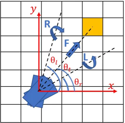
these paths. If one of these paths intersects with an obstacle, the negative reward from the en-vironment will cause the action-value function of these actions to decrease, and consequently, diverging from these paths. In order to determine which actions should be given higher initial values at each state, figure 3.6 is analyzed.
Figure 3.6:The preference is given to a specific action depending on the orientation of the robot
The target orientationθt is defined by the angle between the horizontalxand the line drawn
between the robot COM and the target. If the robot orientation is the same asθt, the optimal
action to be taken is the move-forward action. On the other hand, if the robot orientation is on the left of this line (θl >θt), taking a turn-right action will adjust the robot orientation to align
with the line. Similarly, if the robot orientation is on the right of this line (θr<θt) the optimal
action to be taken is the turn-left action. The assignment of biased initial values can be done by the following pseudo-code:
Result:Biased initialq0 Initializext ar g et;
Initializeyt ar g et;
forevery (x,y,θ) statedo
θt ar g et=t an−1(yt ar g et−y/xt ar g et−x) ; e=θt ar g et−θ;
ife == 0then
q0[(x,y,θ),F]>>0; end
ife < 0then
q0[(x,y,θ),L]>>0; end
ife > 0then
q0[(x,y,θ),R]>>0; end
end
Algorithm 1:Assigning biasedq0for actions at each state (x,y,θ).
CHAPTER 3. PROBLEM ANALYSIS 27
3.2.2 Learning rateαselection
The learning rateαis used to give a desired weight to the recent rewardRover the past re-wards represented in the previous action-valueQ(S,A) while updating it, as shown in figure 3.4. This learning rate takes a values between 0 and 1 (α∈[0, 1]) such that the larger the value, the more the weight given to the recent expected return (R+γmax|a[Q(s0,a0)]) over the
pre-viousQ(S,A) and vice versa. In the case where the stochastic process is non-stationary, the environment supplies a variable rewardr(t) to the learning agent if the same actiona is ap-plied at the same states. This means that this reward changes with time and the learner has to track its change. To achieve that, the most recent received reward must have higher weight over previous rewards, so the learning rate must take a high value (≈1). In the context of the navigation problem where the environment is static, the stochastic process can be considered stationary. However, in the beginning of the learning process, since the algorithm starts from arbitrary initial valuesq0, the received rewards must have high weights overq0. Therefore, in the beginning of the learning process, the learning rateαis set to a huge value. Then, if the learning agent starts reaching an approximate optimal action-valuesq∗, the learning rateα
can be adjusted to a lower value to filter the effect of faulty rewards. In the autonomous navi-gation problem, faulty rewards can occur due to mis-classifying free and obstacle states or due to skidding effects. Thus, the idea of decreasing the learning rateαwith time can limit these effects on the optimal action-valuesq∗. Algorithm 2 shows how to adjust the value ofαwhen the action-valuesQ(S,A) getting close their optimal values. This is detected if the change in their values after the numerical updateδis less than a thresholdθfor each (S,A) pair.
Result:Adjusted learning rateα
Initializeα; Initializeθ; Initializeδ;
Initialized i scount_f ac t or; whileTruedo
δ= min (Q(S,A)−Q(S,A)pr ev,δ);
ifδ<θthen
α∗ =d i scount_f ac t or; end
end
Algorithm 2:Assigning biasedq0for actions at each state (x,y,θ). 3.2.3 Discount rateγselection
The discount rateγgives a desired weight between the effect of the current rewardRand the effect of future rewards encoded in the value of the next stateV(S0)=max|aQ(S0,a) on the update of the current action-valueQ(S,A) as shown in figure 3.4. This parameter can be set be-tween 0 and 1 (γ∈[0, 1]). Since the target of the reinforcement leaning problem is to maximize long-term rewards, this parameter is usually set to a high value to encourage moving to states with higher optimal valuesV∗(s0). For the purpose of accelerating the learning in navigation problems, this parameter must be set to a huge value (≈1), specially in the case of sparse re-ward shaping where all free states give a 0 rere-ward (R=0). In this case, the learner can depend more on the value of the next stateV(S0)=max|aQ(S0,a) to update the value ofQ(S,A) because
a zero reward will not cause any update to its value. 3.2.4 Exploration factor²selection
The Q-learning algorithm can only converge if every state-action pair is visited at least once during the learning process. Therefore, the exploration is an inherent requirement for any re-inforcement learning algorithm. At each state, selecting the most optimal action according to
the current q-values is denoted byexploitationand this exploitation policy is called thegreedy policyπ∗(s). On the other hand, it is required to visit new state-action pairs in the state-action spaces, by selecting actions randomly with probability²resulting in adopting the²-greedy pol-icy. For navigation tasks in an unknown environment, the exploration factor²must have high value in the beginning of the learning process for the following two reasons:
• It helps to discover various parts of the state space till finding states that supply the (pos-itive) reward.
• It helps to build a more accurate model for the state transition probabilities of the system needed to implement a model based Q-learning (section 2.2).
Since the navigation environment is assumed to be static, it is advisable to decease the explo-ration rate with time after the action-value functions are getting close to their optimal values
q∗(s,a). This can be done by multiplying the exploration factor²by a discount factor. This re-duction happens after each episode termination or after discovering a shorter navigation path to the target location as shown in algorithm 3 in section 4.1.2. This approach is denoted by
discounted²-greedy. Finally, in the literature several approaches are described to optimize or to direct the exploration some of which are described in the subsections below.
Softmax action selection
One drawback of the²-greedy method is that it explores equally among all actions[28]. The softmax method varies the action probabilities as a graded function of estimated value. The greedy-action will be given highest probability, but all others are ranked and weighted accord-ing to their Q-value. One of these softmax action selection rules uses a Gibbs, or Boltzmann, distribution. It assigns to each actionaa probability according to the following rule
P(α)= e Q(α)/τ
P
eQ(b)/τ (3.4)
whereτis a positive parameter called the temperature andbdenotes each non-greedy action. High temperatures cause the actions to be nearly equi-probable. Low temperatures cause a great difference in selection probability of actions according to their Q-values.
Directed exploration method
This method aims to direct the exploration towards more interesting areas in the state-action space instead of treating all non-greedy actions equally [4]. An exploration bonus is added to the Q-values to reflect the added value of selecting this action for the sake of exploration. Thus the Q-value for each state-action pair is modified to be
Q+(s,a)=Q(s,a)+ηpm(s,a)/n(s,a) (3.5) where ηis a constant, m(s,a) is the number of time steps since action a was last tried in
s. n(s,a) is the total number of trying a ins. Then, this modified Q-value is substituted in Boltzmann distribution (3.4) to assign probabilities of selecting each action. Such a method is proven to be beneficial while depending on based Q-learning [4]. Otherwise, model-based Q-learning algorithms converge to sub-optimal policies. For this reason, it seems to be a promising exploration strategy for the navigation problem.
3.3 Dyna-Q-based navigation
Q-learning algorithm is amodel-freereinforcement learning algorithm since it depends only on the learning to update action value functions for each state-action pair. On the other hand,
significantly large as in autonomous navigation problems. In order to show the potentials of the Dyna-Q algorithm, it has been simulated for the grid-world problem as shown in figure 3.8. Unlike the standard Q-learning that takes about 80 episodes to converge, it converges really fast in 7 episodes. The results of applying it to real navigation tasks are discussed in chapter 5. 3.3.1 Necessary adjustments to the navigation problem
The general Dyna-Q algorithm presented in [27] assumes a deterministic dynamical environ-ment. However, in the context of autonomous navigation for SSMRs, sliding is an inherent system property that leads to stochastic dynamics. Thus, it is required for the learned model to be probabilistic. The basic idea is to learn a model that does not predict a deterministic next state and a deterministic reward, but a probability distribution over next states and next rewards [27]. For discrete finite MDPs, it is possible to represent the state transition probabili-tiesp(s0,r|s,a) using multinomial distributions [14]. The design of the algorithm to learn these multinomial distributions is presented in section 4.1.2. However, it should be noted that the online-constructed models can never represent the navigation environment identically espe-cially if a limited number of samples have been observed. When the model is inaccurate, the planning process will compute sub-optimal policies [28]. Using these multinomial models, it is only possible to simulate hypothetical experiences for already-visited state-action pairs (s,a). If it is required to predict probability distributions for the next states and rewards for state-action pairs that have not been visited before, an accurate model for the robot motion must be developed. Possibilities to construct this motion model for SSMRs depend on their motion characteristics that will be analyzed in the following section.
[image:36.595.184.382.423.630.2]3.4 Motion analysis of Skid-Steering-Mobile-Robots
Figure 3.9:SSMR free body diagram [13].
The kinematic model for SSMRs has been explained in section 2.5. The generalized velocity (figure 3.9) equation can be described by:
˙
X
˙
Y
˙
θ
=
cos(θ) −si n(θ) 0
si n(θ) cos(θ) 0
0 0 1
vx vy ω
CHAPTER 3. PROBLEM ANALYSIS 31
The vector [vxvyω] represents the car velocity in its local reference frame. This velocity vector
is related to the wheels angular velocity by the following equation:
·
vx ω
¸
=r
· ωL+ωR
2 −ωL+ωR
2c
¸
(3.7)
andvyis constrained by the rotation of the robot and can be expressed by the following
equa-tion:
[image:37.595.202.396.230.421.2]vy+xIC Rθ˙=0 (3.8)
Figure 3.10:Velocities of one wheel [13].
The model represented by equation 3.7 assumes that the longitudinal slip is not dominant in the robot motion. This assumption is no longer valid if the robot is navigating above slippery surfaces. To understand the effect of the slippage on the wheels motion, figure 3.10 is analyzed. The velocity of the wheel in the longitudinal directionvi xdepends only on the rotation of the
wheelωiin case of a pure rolling. However, if the wheel slides, the termlongitudinal wheel slip λiis defined to fully describe the wheels motion in the longitudinal direction [18]:
λi=
vi x−rωi vi x
(3.9) This longitudinal wheel slip depends on the normal force acting on the wheel, the road surface conditions and tire characteristics [19]. In [1], the relation between the longitudinal wheel slip and the friction coefficient is analyzed.
![Figure 2.1: The agent-environment interaction in a Markov decision process [28].](https://thumb-us.123doks.com/thumbv2/123dok_us/9662025.468189/16.595.156.415.257.349/figure-agent-environment-interaction-markov-decision-process.webp)
![Figure 2.5: The tabular prioritized sweeping algorithm [28].](https://thumb-us.123doks.com/thumbv2/123dok_us/9662025.468189/20.595.94.475.236.451/figure-the-tabular-prioritized-sweeping-algorithm.webp)
![Figure 2.6: SSMR free body diagram [13].](https://thumb-us.123doks.com/thumbv2/123dok_us/9662025.468189/22.595.182.380.479.666/figure-ssmr-free-body-diagram.webp)
![Figure 2.8: Wheel velocities [13].](https://thumb-us.123doks.com/thumbv2/123dok_us/9662025.468189/23.595.205.397.190.396/figure-wheel-velocities.webp)
![Figure 3.9: SSMR free body diagram [13].](https://thumb-us.123doks.com/thumbv2/123dok_us/9662025.468189/36.595.184.382.423.630/figure-ssmr-free-body-diagram.webp)
![Figure 3.10: Velocities of one wheel [13].](https://thumb-us.123doks.com/thumbv2/123dok_us/9662025.468189/37.595.202.396.230.421/figure-velocities-of-one-wheel.webp)
![Figure 3.11: Longitudinal slip as a function of friction coefficient [1].](https://thumb-us.123doks.com/thumbv2/123dok_us/9662025.468189/38.595.124.447.72.256/figure-longitudinal-slip-function-friction-coefcient.webp)