Modelling the influence of sand mud interaction and waves on salt marsh development

“MODELLING THE INFLUENCE OF

Modelling the influence of sand-mud interaction and waves

on salt marsh development

Master thesis in Civil Engineering and Management

Faculty of Water Engineering and Technology

University of Twente

Author: Wouter Vreeken

E-mail: [email protected] Location and date: Rotterdam, July 10, 2015 Thesis defence date: July 17, 2015

Graduation committee:

Ir, B. Van Leeuwen (Bas) Svašek Hydarulics

E-mail: [email protected] Telephone: 010 467 1361

Dr. Ir. B.W. Borsje (Bas) University of Twente

E-mail: [email protected] Telephone: 053 489 3546

Direct line: 053 489 1094

Prof. Dr. S.J.M.H. Hulscher (Suzanne) University of Twente

E-mail: [email protected] Telephone: 053 489 3546

PREFACE

This thesis is about modelling the influence of sand-mud interaction and waves on salt marsh development. I made this thesis at Svašek, a hydraulic engineering company located in Rotterdam. During my research I worked with FINEL2D (model developed by Svašek) which increased my modelling skills. In addition, I gained more knowledge about salt marshes and processes influencing salt marsh development.

I would like to thank my supervisors. First I would like to thank Bas van Leeuwen, my daily supervisor at Svašek. Whenever I had questions he was able to answer them. Furthermore I would like to thank him for his enthusiasm during my research. I would also like to thank Bas Borsje, my daily supervisor at University of Twente. He really helped me structuring my research and supported me with suggestions. I would also like to thank Suzanne Hulscher for her critical view during our meetings.

I would also like to thank all staff at Svašek. I had a lot of pleasure working there and especially our “spelletjesavonden” were a lot of fun. In addition I would like to thank Bram van Prooijen for his advice during our meeting.

ABSTRACT

Sea level rise requires innovative solutions in flood protection. Salt marshes could be such a solution because of their adaptive ecological characteristics. Salt marshes are tidally influenced ecosystems between land and sea. They attenuate waves and decrease fetch length. In addition, salt marshes are able to capture sediment and rise in elevation, making it an effective flood protection. The recent interest in salt marshes leads to questions and this thesis therefore analyses the significance of different processes in salt marsh development. This could eventually help in maintenance of current marshes but also in the construction of artificial marshes.

FINEL2D is used for analysing long-term development of salt marshes. FINEL2D is a depth-average numerical model developed by Svašek Hydraulics. With the use of FINEL2D, 100 years of salt marsh development is simulated. The dimensions of the test case are based on

Paulinaschor, a relative small salt marsh located in the Western Scheldt, Netherlands. First a simulation is done with sand as only sediment fraction. Then the interaction between sand and mud was implemented in the model. Sand and mud show cohesive behaviour when a certain percentage of mud is present in the soil. This cohesive behaviour leads to higher critical shear stresses. Finally plants were added. Vegetation influences flow velocities as higher plant densities cause more friction. Also growth and decay of vegetation is present in FINEL2D. The simulation with vegetation in combination with sand-mud interaction functioned as reference simulation to compare with adapting processes. Results show that the implementation of mud is essential for a salt marsh environment to arise. Mud leads to significant higher bed levels due to settling lag. Plants establish on locations where no creeks are present. Vegetation determines the creek pattern as plants obstruct flow leading to more creeks which are needed to discharge all water after high tide.

Validation of results showed similarities with Paulinaschor. The height of the marsh platform and the location of the marsh edge correspond well with Paulinaschor but there are also some differences. The simulations showed a marsh edge of about 4 meters high as there is no mudflat. Paulinaschor has an edge of 2 meters high. This difference could be caused by only taking two sediment fractions in consideration. Therefore is recommended to further research the effect of implementing multiple sediment fractions.

The following processes are evaluated: tidal amplitude, mud availability, critical deposition shear stress (continuous deposition), critical mud content (determines when bed is cohesive), settling velocity and maximum bottom slope. The availability of mud determines lateral expansion of the marsh, while tidal amplitudes influence the expansion of the marsh but also the height. Because of high critical shear stresses sediment is able to constantly deposit and this results in an extended marsh towards the channel. The effect of a lower critical mud content was minimal, however, also this simulation showed a slight expansion compared to the reference simulation. When a low settling velocity for mud was implemented, mud was not able to settle and a small salt marsh arose. Nevertheless, the simulation with low settling velocities was the only simulation which shows higher mud percentages with distance from the channel. With a maximum bottom slope is meant that when a certain slope is reached, erosion occurs according to avalanche formulations. In this simulation a maximum bottom slope of 0.5 is applied. This results in erosion of the marsh edge. All simulation show establishment of plants over the entire marsh platform except for locations where creeks are present.

CONTENT

1 Introduction 9

1.1 Problem definition 10

1.2 Research objective 10

1.3 Research questions 11

1.4 Report outline 11

2 Salt marsh dynamics 12

2.1 What are salt marshes? 12

2.2 Sand-mud interaction 13

2.3 Processes influencing salt marshes 14

3 Model set-up 18

3.1 Model description 18

3.2 Model area 20

3.3 Boundary conditions 21

3.4 Input parameters 23

3.5 Analysis set up 25

3.6 Evaluation methods 26

4 Results and validation 27

4.1 Bed level 27

4.2 Plants 30

4.3 Mud content 31

4.4 Validation 31

5 Sensitivity analysis 33

5.1 Process descriptions 33

5.2 Results 34

5.3 Summary 41

6 Exploring storm effects 43

6.1 Wave input 43

6.2 Results 44

7 Discussion 50

7.1 Discussion of methodology 50

7.2 Construction of artificial salt marshes 51

8 Conclusion 53

8.1 Which processes contribute to salt marsh development according to literature? 53 8.2 How can sand-mud interaction be taken into account when simulating salt marsh

development? 53

8.3 How can the influence of storms on salt marshes be modelled? 53

8.4 How can the marsh model be validated? 53

8.5 What is the influence of the following processes on salt marsh development? 53

9 References 55

1.1 Sand-mud interaction 60

1.2 Multiple layer mixing 61

1.3 Vegetation 62

1.4 Storm events 63

2 Appendix: Soil characteristics Paulinaschor 64

3 Sensitivity model 65

4 Appendix: Bed level development 68

5 Appendix: Plant densities 69

List of symbols

Plant drag coefficient [-]

Bed-friction coefficient [-]

Erosion rate of mud [ ]

Erosion coefficient cohesive [ ] Erosion coefficient non-cohesive [ ]

Morphological adaptation time [ ] Equilibrium concentration [ ]

Median grain size [ ]

Plant density [ ]

Mud content [-]

Settling velocity [ ] Dry bulk density of sediment [

Density of water [

Bed shear stress [ ]

Critical bed shear stress [ Critical sedimentation shear stress [

Water depth [ ]

Chézy coefficient [

Sediment concentration [ ] Acceleration of gravity [ Vegetation stem height [ ] Depth-averaged velocity [ ]

Porosity [-]

1

INTRODUCTION

The Dutch have a long history of defending against water. Because 26% of the Netherlands is below mean sea level this challenge is still a hot topic. For a prolonged period the policy was to construct hard solutions to defend land from water. Nowadays interest also goes out to dynamic measures, especially ecological measures. The study of “ecological engineering” attempts to integrate ecology and engineering into flood-protecting solutions .These measures promise cost-effectiveness and sustainability. Furthermore there is a need for solutions which minimize human impact on ecosystems (Borsje et al., 2011). These solutions can be implemented in two ways: the first is by adapting current hard structures, the second by implementing entirely new ecosystems. Ecosystems are locations where living organisms and non-living components interact with and influence each other. Systems which are able to trap sediments can therefore be considered ecosystems. Examples of these kinds of ecosystems are salt marshes, mussel beds and mangroves.

Constructing salt marshes is a good example of ecological flood protection and anti-erosion measure. Salt marshes are coastal ecosystems which are located along the sea and are

regularly flooded by salt water (see figure 1). In general, salt marshes inundate during flood while during ebb tide the marsh dries. During flood sediments are transported towards the salt marsh. When flooded, flow velocities decrease and sediments are able to settle. The settlement of sediments leads to increased bed levels on the marsh. This positively influences wave attenuation (Möller & Spencer, 2002). Furthermore, salt marshes also tend to expand laterally and thereby decrease the fetch of waves (Bouma et al., 2005).

FIGURE 1 LAND VAN SAEFTINGHE, SALT MARSH IN THE WESTERN SCHELDT, NETHERLANDS

example Temmerman (2005) did a study on the relative impact of different processes on the spiral flow and sedimentation pattern in a tidal marsh landscape. He found that vegetation has the strongest control on flow routing and spatial sedimentation pattern during single inundation events. However, he did not study the long-term effect of vegetation. In addition, no study has yet been undertaken which combines the effect of multiple sediment fractions with the effect of vegetation-related processes.

New insights in salt marsh development could provide recommendations towards salt marsh maintenance and could also be useful in constructing artificial marshes. This thesis can contribute to defining the influence of processes in the development of salt marshes, which improve the construction of artificial salt marshes.

1.1 Problem definition

Many processes affect salt marsh development. Hydrodynamics cause marshes to inundate, morphological process lead to sedimentation of marshes and vegetation influences salt marsh patterns. These processes also influence each other which make salt marshes complex ecosystems. In order to evaluate different processes, FINEL2D is used. FINEL2D is a depth-average numerical model developed by Svašek Hydraulics and already has a lot of these processes included (Dam et al., 2014). However, the effect of interacting sand and mud fractions in combination with vegetation-related processes on the development of salt marshes has not yet been studied. Modelling marsh development can contribute to understanding the different

processes. Models are capable of assessing the influence of different processes by isolating the effects of different input.

In the past years there has been an increase in knowledge about modelling salt marsh

development. Examples of these advances are the incorporation of hydraulic roughness induced by vegetation (Baptist, 2005; Klopstra et al., 1997) but also vegetation dynamics (growth and decay of vegetation) (Balke et al., 2011; van Wesenbeeck, 2007).

Temmerman (2005) has conducted a study on the relative impact of different processes on the spiral flow and sedimentation pattern in a tidal marsh landscape. Attema (2014) extended the study of Temmerman by including the window of opportunity model developed by Balke (2011). The window of opportunity model simulates growth and decay of vegetation. Attema concludes that in a system where vegetation is leading the morphological development

bio-geomorphological modelling (simulating of vegetation establishment and growth in interaction with geomorphological- and hydrodynamic processes) is very important. Attema undertook a case study on the “Land van Saeftinghe”, a salt marsh located in the Western Scheldt. Although the model was able to simulate the major creeks system and lateral extension, he still found some differences between the model and the actual development of the marsh. The model was not capable of predicting the exact bed level elevation. Attema states that this difference in bed level elevation could be the result of taking only one sediment fraction into account. For the “Land van Seaftinghe” case study an unrealistic fine sand fraction was used causing sand to settle on high locations. The grain size of mud is lower and therefore implementing mud could tackle this problem. Mud in combination with sand can form a cohesive mass which makes the bed hard to erode. More about the interaction between sand and mud is presented in chapter 2.2.

1.2 Research objective

The objective of this report is to evaluate the contribution of hydrodynamic,

morphological and vegetation processes on the overall development of salt marshes.

based on bed level, mud content and vegetation. In addition an initial step towards modelling salt marsh development in combination with storm events is executed.

1.3 Research questions

The overall aim of this thesis is to evaluate the importance of different processes contributing to salt marsh development. To reach this goal the following sub questions are addressed.

1. Which processes contribute to salt marsh development according to literature? 2. How can sand-mud interaction be taken into account when simulating salt marsh

development?

3. How can the influence of storms on salt marshes be modelled? 4. How can the marsh model be validated?

5. What is the influence of the following processes on salt marsh development? a. Sand-mud interaction

b. Vegetation c. Tidal amplitude d. Mud availability e. Continuous deposition f. Settling velocity mud g. Critical mud content h. Maximum bottom slope i. Storms

1.4 Report outline

This report is structured as follows: chapter 2 provides theory of this research. First a brief description of salt marshes is presented followed by the interaction of mud and sand. Then processes influencing salt marsh development are described. Chapter 3 provides the set up of a test model. In this chapter the model area, boundary conditions and input variables are

described. Furthermore this chapter provides information of different processes which will be examined. The last paragraph of chapter 3 shows how simulation results are analysed.

2

SALT MARSH DYNAMICS

This chapter provides a definition of salt marshes and processes affecting marsh development. Also a description of sand-mud interaction is provided.

2.1 What are salt marshes?

Salt marshes are tidal-influenced ecosystems usually located at the seaward side of the dike. Salt marshes only occur at low-energy shorelines in temperate and high latitudes (Allen & Pye, 1992) and are formed on sheltered locations where fine sediments can settle (Fagherazzi et al., 2012). During high tide the marsh becomes inundated while during ebb tide the marsh remains dry. Therefore salt water enters the marsh during high tide and vegetation located on the marsh has to withstand salty inflow. This unique environment makes salt marshes one of the richest ecosystems in terms of productivity and species diversity (Tonelli et al., 2010). Typical locations of salt marshes are estuaries, shallow bays and landward sides of barrier islands. Salt marshes can also arise at large rivers and deltas, but only when enough sediment is available for

formation and evolution.

Salt marshes consist of multiple sections with each their own characteristics considering inundation frequency and vegetation species. Lower marshes, located at the sea boundary inundate every flood tide and consist of other plants than high marshes, which only inundate during above average high tides. Figure 2 shows a cross-section with different sections of a salt marsh with their corresponding vegetation types.

FIGURE 2 CROSS-SECTION SALT MARSH SHOWING DIFFERENT SECTIONS

FIGURE 3 DIFFERENT SALT MARSH VEGETATION UPPER LEFT: SPARTINA ALTERNIFLORA. UPPER RIGHT: SALICORNIA. BOTTOM LEFT: LAVENDER. BOTTOM RIGHT: RUSHES

After pioneer vegetation has established, sedimentation occurs. Erosion of marsh edges are generally linked to erosion by wind waves (Van De Koppel et al., 2005; Möller, 2006; Möller et al., 1999). Most marshes have a steep scarp dividing salt marsh and tidal flat (Mariotti &

Fagherazzi, 2010; Van De Koppel et al., 2005). Because salt marshes are constantly influenced by tides and wind waves they change depending on sedimentation rates and wave erosion (Fagherazzi et al., 2007). Equilibrium in bed levels for waves is reached when the energy generated by wind action equals dissipated energy. However, the most important factor in stability of a dynamic equilibrium is the availability of sediment (Fagherazzi et al., 2006). If sediment availability increases, more sediment is deposited resulting in higher bed levels.

2.2 Sand-mud interaction

Whether a particle is classified as mud or sand depends mostly on grain size. Grains are classified as sand when their size ranges between 2 mm and 62.5 μm. The grain size of mud particles is everything smaller than 62.5 μm. The influence of mud in combination with vegetation on a developing salt marsh is not extensively examined yet. However, the contribution of mud on the development of salt marshes is quite significant. Mud affects bed levels and thereby water levels and vegetation patterns. Before addressing how mud is introduced in the model, the contribution of mud in salt marsh development is qualitatively assessed.

Van Ledden (2003) analysed the grain size distribution of the Western Scheldt. The median grain size in the Western Scheldt is 157 μm. A grain size of 157 μm is classified as fine sand. Although the median grain size of the Western Scheldt corresponds with fine sand, there is a relative large percentage mud present in the soil (44.3%). Although these values differ locally it tells us at least that there is plenty of mud available which can influence salt marsh development.

A comprehensive process-based model in which mechanisms are brought together to explain large-scale sand-mud segregation did not exist until van Ledden (2003) developed a method in which the interaction between sand and mud is described. High percentages of mud have consequences on deposition and erosion. When 5% to 10% of clay (median grain size between 1 μm and 4 μm and therefore identified as mud) is present in the soil it becomes cohesive. A cohesive bed is more difficult to erode due to electrostatic forces between smaller mud particles. Sand can be “trapped” in such a cohesive bed. A cohesive bed leads to a higher critical bed shear stress and therefore larger velocities are needed for erosion. To determine whether the bed is cohesive or not Van Ledden (2003) developed a method based on a critical mud content. When a certain percentage of mud is present in the soil, the bed becomes cohesive. In the Netherlands generally 30% of mud is used as a transition value from a non-cohesive to cohesive bed (Van Ledden, 2003).

The cohesiveness of soils affects accretion rates because erosion is less likely to occur. The highest accretion rates are observed at the salt marsh boundary as here the frequency of inundation is largest (Détriché et al., 2011). Towards the upper marsh accretion rates decrease as this part of the marsh is less inundated than the boundary. Zwolsman et al. (1993) analysed the accretion rates for the Western Scheldt marshes and found values of approximately 1.3-1.7 cm/year for Land van Saeftinghe and for Emanuelpolder 0.84-0.90 cm/year. These salt marshes also experience cohesive behaviour of the soil. However, they did not quantify this effect. The implementation of sand-mud into FINEL2D is described in appendix 1.

2.3 Processes influencing salt marshes

In figure 4 different processes affecting salt marsh development are presented in a schematic way. The four main processes are hydrology, vegetation, waves and sediment transport plus bed level update. The interaction between sand and mud is classified as sediment transport. The arrows in the figure indicate that these processes, next to affecting salt marshes, also affect each other. In this chapter vegetation-related processes are described. The numbers in the figure indicate the paragraph in which the specific interaction is discussed.

2.3.1 Vegetation  hydrology

There has been a lot of research on the effect of vegetation on water-influenced ecosystems in the last few years. These studies resulted in the set up of different vegetation models. Vegetation influences the development of salt marshes in a few ways. One of these ways is the influence on flow velocities. Dense vegetation lets flow velocities decrease. This reduction in flow velocity depends on the density, height and stem diameter. The effect of plants on flow velocities is quantified in the hydraulic roughness. Figure 5 shows a representative situation of the effect of vegetation on velocities in the water column.

FIGURE 5 VELOCITY PROFILE OF SUBMERGED VEGETATION. K IS VEGETATION HEIGHT, U(Z) IS VELOCITY AND H IS WATER LEVEL

There are different methods which translate vegetation to a representative hydraulic roughness. In the Netherlands there are two methods which are used. The first method is developed by Klopstra et al. (1997). This method requires the following characteristics of vegetation to

calculate the hydraulic roughness: stem diameter, stem density and vegetation height. The other method is set up by Baptist (2005). The method of Baptist requires the same vegetation

characteristics but is a bit less complex. The main difference between the method of Klopstra and Baptist is that the method of Baptist is made dependent on the turbulence intensity near the bed. The underlying idea of this assumption is that the shear stress profile near the bed is not so much affected by drag forces of sediment particles alone, but by a combination of drag forces of sediment and vegetation. Although these methods differ from each other in calculating the hydraulic roughness, their principle is the same. When stem diameter increases, the incoming wave or current experiences a bigger friction surface. This leads to a larger wave or current energy dissipation. The stem density of plants influences waves and currents in the same way as the stem diameter. Vegetation height also affects the flow as velocity through and over

vegetation differs from a normal velocity profile.

2.3.2 Hydrology  vegetation

Besides the effect of vegetation on hydrodynamics, there is also an effect reverse. This effect of hydrodynamics on vegetation is called “vegetation dynamics”. Hydrodynamic properties of a flow determine whether vegetation establishes or decays. In past recent years this effect got more attention which resulted in different methods. In this chapter two of these methods are discussed.

vegetation is meant that vegetation is able to expand to surrounding locations. The expansion rate depends on the difference in density between two adjacent locations and growth rate.

The other method is called the window of opportunity model by Balke et al. (2011). The biggest difference between the population dynamics model and the window of opportunity model is that vegetation in the window of opportunity model can only establish when favourable conditions are present while in the population dynamics model vegetation can establish everywhere and afterwards is analysed whether this location fulfils favourable conditions for vegetation to further develop.

Before vegetation establishes and develops into permanent vegetation in the window of opportunity model, it has to withstand three stages. The first stage requires an inundation free period. When this requirement is fulfilled, vegetation can establish based on a stochastical function. In the second stage the root system develops. For this stage to happen a relative calm inundation period is required. This stage is important for vegetation to develop their roots and thereby increase their resistance. After the root system reaches maturity, seedlings need to survive extreme energy events like spring tide or storms. When seedlings also survive this stage, stem density grows and vegetation expands according to the same principle as in the population dynamics model.

The window of opportunity model does not consider any decay processes, but monitors the conditions of existence of vegetation. These conditions are specified in terms of inundation period and bed shear stresses. When one of these conditions is not met, vegetation decays.

Attema (2014) compared these two vegetation dynamics methods and concluded that the outcome does not differ significantly. However, the window of opportunity model is better in describing the actual development of vegetation as in this model plants can only establish on locations where conditions are favourable whereas in the population dynamics model vegetation establishes everywhere and afterwards is analysed whether the conditions are favourable. Because the development of vegetation is better described by the window of opportunity model, this method is used in this research. The implementation of this model is described in appendix 1.

2.3.3 Vegetation  sediment transport + bed level update

Another aspect of vegetation is the ability to trap sediments. The amount of sediment that is trapped depends on the surface roughness of stems and leaves (Yang, 1998). When currents and waves flow through plants, part of the energy is dissipated by stems and leaves of

vegetation. This results in a decrease in velocity and wave height. This decrease in velocity and wave height affects the capacity of water to carry sediment and thereby deposition rates.

Vegetation influences the stability of the soil in two ways: through hydrological effects and mechanical effects (Chok et al., 2004). Hydrological effects involve evapotranspiration of water from the soil through plants. Evapotranspiration by plants reduces the amount of water in the soil resulting in higher soil shear strength. Shear stresses are also affected by mechanical effects of plants. The density and tensile strength of the roots contribute to the ability of the soil to resist shear stresses. The increasing stability of the soil is only indirectly modelled as the hydraulic roughness increases by plants and therefore the soil becomes more resistant for shear stresses. However, these equations do not include root density, tensile density by roots and change in porosity of the soil. The question remains how big the influence is of these processes. A new study has to be set-up in order to quantify this effect.

2.3.4 Sediment transport + bed level update  vegetation

Large erosion rates cause roots to be exposed to the surface. Exposure of roots leads to

decreased plant stability (Osterkamp et al., 2012). In addition, erosion also leads to a decrease in water and nutrient uptake from plants and thereby reduces their vitality. This reduction in vitality is caused by dieback from a cellular plant tissue which is responsible for creating new cells (Carrara & Carroll, 1979).

This effect is not implemented in the model. However, large erosion rates most come hand in hand with high shear stresses. Decay by high shear stress is present in FINEL2D. Although low erosion rates over a long time span could cause roots to be exposed to the surface. This would lead to wash out of plants.

2.3.5 Vegetation  waves

Vegetation dissipates waves due to the morphology, stiffness and length of vegetation (Houwing et al., 2002). Not only the characteristics of plants determine the dissipation of wave energy, also wave properties are important. However, the density and height of plants contribute the most to wave dissipation.

2.3.6 Waves  vegetation

In the window of opportunity model, waves are not included. However, there is a model which includes the effect of waves on vegetation. Vegetation damage by waves is assumed to be a linear function of the slope in sediment elevation and a conversion constant (Koppel et al., 2005). The slope in sediment elevation is important for the damage by waves because the slope

determines the length and height of exposure.

3

MODEL SET-UP

3.1 Model description

As already stated in the problem definition, the modelling software primarily used in this thesis is FINEL2D (FINite Element 2Dimensional). FINEL2D is able to simulate flows in rivers, estuaries, lakes and coastal waters. Because FINEL2D contains a robust procedure for drying and flooding of tidal flats, it is especially suited to model the interaction between flow and morphological characteristics in estuaries.

The biggest difference between other software packages and FINEL2D is that the model domain is divided into triangles instead of rectangles. These triangles are called elements. The element size can be specified beforehand. In this way modelling time can be adapted and more detail can be applied on specific locations of interest. The shallow water equations are then solved for each element.

In FINEL2D there are four sorts of model types. Each model type corresponds with a specific calculation. FINEL2D is able to compute flow, flow and mud, flow and sand and flow including the interaction between sand and mud. The latest development in FINEL2D is the introduction of vegetation effects. By turning on the plant switch the effect of vegetation on the hydraulic roughness can be analysed. Also the effect of vegetation dynamics (growth and decay) can be modelled.

FIGURE 6 SCHEMATIC OVERVIEW OF FINEL2D

transport module. In addition, hydrodynamic conditions (inundation time and bed shear stress) are constantly monitored to assess whether conditions are favourable for plants to establish, develop or remain present. Once not favourable, vegetation decays.

To reduce simulation time, a morphological acceleration factor is used. The erosion and deposition rates calculated in the sediment transport mode are multiplied by this factor. This means that when for example a hydrological time step of 5 seconds is simulated, a

morphological acceleration factor of 25 results in a bed level update of 125 seconds. This is an effective and simple way of decreasing simulation time.

After the deposition rates and erosion rates are multiplied by the morphological acceleration factor, the bed is updated and the cycle starts over again as the new bed has consequences for the hydrodynamic model. The implementation of sand-mud interaction, multiple layer mixing and vegetation are discussed in appendix 1.

When the effect of waves are analysed SWAN is used. SWAN is a wave model for obtaining realistic estimates of wave parameters in coastal seas, lakes and estuaries developed by Delft University of Technology. SWAN and FINEL2D are already linked to each other. The waves in SWAN are translated into wave forces. Wave forces then influence the hydrodynamic model of FINEL2D. FINEL2D influences waves by water levels and currents. FINEL2D as SWAN each deliver a shear stress for the sediment transport model of FINEL2D. These shear stresses are then added resulting in the total shear stress used as input for calculating sediment transport. The combined shear stress is also used for monitoring vegetation dynamics conditions. In the current model the shear stress induced by waves was not linked to vegetation. Therefore FINEL2D had to be adapted (see appendix 1).

3.1.1 Overview processes in FINEL2D

In table 1 the implementation of processes mentioned in chapter 2.3 in FINEL2D is presented

TABLE 1 IMPLEMENTATION OF PROCESSES INTO FINEL2D

Process Implementation

Vegetation  hydrology

- Flow hindrance Method of Baptist (2005) with increased roughness

Vegetation  sedimentation + bed level update

- Increased capture of fine sediment by stems and leaves

Not implemented

- Increased soil stability by

evapotranspiration through plants

Not implemented

- Prevent erosion due to soil stabilization by roots

Not implemented,

Hydrology  vegetation

- Vegetation dynamics Window of opportunity model (Balke et al., 2011)

Sediment transport + bed level update  vegetation

- Large erosion digging out roots Not implemented, indirectly through high shear stresses in the window of opportunity model Vegetation  waves

- Wave attenuation Not implemented

Waves  vegetation

3.2 Model area

A test case area is set-up to evaluate different processes. The area used in this test case is based on dimensions of Paulinaschor. Paulinaschor is a salt marsh located in the Scheldt estuary at the west of Terneuzen (see figure 7).

FIGURE 7 PAULINASCHOR, NETHERLANDS. THIS MARSH IS USED AS BASIS FOR THE TEST CASE

One of the reasons for choosing dimensions of Paulinaschor as test case is the size of this salt marsh. Paulinaschor is a relatively small salt marsh. The advantage of modelling a small salt marsh is the short modelling time. Another advantage is that applying proper boundary conditions, a salt marsh should arise. After all, this location also developed into a marsh.

The initial bed profile of the test case is presented in figure 8. The bed level of the channel flowing along the marsh (with marsh is meant the middle section of figure 8) is located five meters below mean sea level (hereafter referred as NAP which is approximately mean sea level in Dutch waters). In front of the marsh a 1:20 slope is applied. This seems a little steep, however simulations showed that this slope does not influence the outcome of the simulations. Another option would be to implement a cliff between the channel and the marsh, but a slope

corresponds physically better with actual marshes. A slope of 1:20 implies that the marsh surface is at mean sea level in the beginning of the calculation. In this way the development from flat bed to a fully developed marsh can be modelled. The channel is relatively wide compared to the marsh. In this way the boundary conditions can adapt to the circumstances in the channel with a more realistic simulation as result. The channel area of the model is 4000 metres long and has a width of 1200 metres. The marsh located at sea level has a length of 300 metres and a maximum width of 1000 metres. The marsh has a minimum width of 200 metres.

FIGURE 8 INITIAL BED PROFILE TEST CASE

FIGURE 9 GRID PROFILE WITH MORE DETAIL ON THE MARSH THAN IN THE CHANNEL

3.3 Boundary conditions

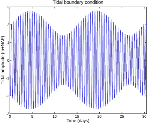
Boundary conditions are imposed at the left, upper and right side of the channel. The hydrodynamic boundary consists of four tidal components: M2, S2, MN4 and S4. These components are chosen in such a way that together they show a spring-neap cycle (advised by Bram van Prooijen). The result is presented in figure 10. In this figure a month of water level variation is presented and the spring-neap cycle is clearly observed. Amplitudes corresponding the individual components are presented in table 2. The amplitude of the M2-tide is assumed to be two metres. By using a database with different tidal components the amplitude of the other three components are based on the relative amplitude in comparison to the M2-tide.

0 500 1000 1500 2000 2500 3000 3500 4000

0 200 400 600 800 1000 1200

x-coordinate (m)

y

-c

oordin

at

e

(m

)

Intial bed level

Bed

lev

el

(m

N

AP)

-5 -4 -3 -2 -1 0

0 500 1000 1500 2000 2500 3000 3500 4000

0 200 400 600 800 1000 1200

x-coordinate (m)

y

-c

oordin

at

e

(m

)

FIGURE 10 TIDAL BOUNDARY CONDITION

TABLE 2 AMPLITUDES OF TIDAL COMPONENTS

Tidal component Amplitude (m)

M2 2.0

S2 0.69

MN4 0.01

S4 0.02

Novel in this study is that the tide does not propagate perpendicular but parallel to the shore, as is normally the case for salt marshes in the Scheldt. The right boundary of the area is located 4000 metres from the left boundary resulting in a phase difference. For calculating phase differences, wave velocities are needed. Tidal waves are shallow water waves in coastal waters Therefore wave-propagation velocities are calculated using . In this equation is water depth in meters, so in this case 5.00 metres, and is the acceleration of gravity, which is equal to 9.81 m/s2. This means that the wave propagation velocity has a value of 7.00 m/s. Dividing the distance from the left to the right boundary (4000m) by the wave propagation velocity (7.00 m/s) provides the time it takes for waves to flow from one end to the other. Dividing this time by the period of the tidal component results in a phase difference. Because FINEL2D requires a phase difference in radians, the outcome has to be multiplied by 2 . In the initial situation the phase on the left boundary is assumed to be zero and on the right boundary the calculated phase

difference is imposed. Because waves move from left to right, the phase difference on the right is negative as it lags waves coming in from the left.

In table 3 each tidal component with their corresponding period and phase difference is presented.

TABLE 3 PHASE DIFFERENCE OF TIDAL COMPONENTS

Tidal component Period (s) Phase difference

M2

44700

S2

43200

MN4 22569 -0.159

S4 21600 -0.166

0 5 10 15 20 25 30

-3 -2 -1 0 1 2 3

Time (days)

T

id

a

l

a

m

p

liu

d

e

(

m

+

N

A

P

)

3.4 Input parameters

FINEL2D requires input parameters considering flowconstants, plants, morphology, time-related input and some general information. The input parameters will be explained in this paragraph.

3.4.1 Roughness

A spatial-varying bed roughness is implemented. Usually a Nikuradse roughness length of 2cm is used. However, at the left and right bottom grid boundaries a high roughness length of 10m is applied (see figure 11). This is done because test simulations showed that when using a Nikuradse length of 2cm for the whole domain, a spiral flow occurs at the boundaries (due to boundary effects) resulting in unrealistic bed level changes.

FIGURE 11 INITIAL ROUGHNESS OF THE GRID IN NIKURADSE LENGTH

3.4.2 Simulation time

A period of 100 years is used in the simulations. As will be seen in the upcoming results, 100 years is long enough for the simulations to reach or come close to equilibrium conditions. Because simulating 100 years takes a lot of time an acceleration factor of 100 is used. This means that every time step, morphological changes are multiplied with 100. Doing so, it takes about three days to simulate 100 years of morphological development.

3.4.3 Morphological active area

In FINEL2D an active morphological zone has to be determined. This means that morphological influences are only present within given boundaries resulting in a shorter simulation time. In this research the boundaries are set in such a way that only around the marsh, morphological changes occur. The values of the boundaries are presented in table 4.

On the boundaries of the morphological active area a mud concentration has to be implemented. According to Veheyen et al.(2013) mud concentrations are around 50 mg/l in the Scheldt estuary. Therefore the boundary concentration is put on this value. The effect of different boundary concentrations is analysed later in this thesis.

3.4.4 Morphological parameters

The values for the sand-, mud- and sand/mud variables in the reference case are based on a paper from Dam and Bliek (2013). Dam and Bliek studied the effect of sand and mud on sedimentation and erosion of a salt marsh located in the Scheldt estuary near Waarde. At Waarde a mud flat is located between two constructed groynes. This tidal mud flat is sensitive for deposition from sand as well as mud. The objective of this study was to assess the quality of the sand-mud module present in FINEL2D. Dam and Bliek conclude that after simulating 5 years, the model is able to produce bed level development. However, the performance of sand-mud

interaction in combination with vegetation on a developing salt marsh has not been studied yet and thereby this research differs from the study by Dam and Bliek.

0 500 1000 1500 2000 2500 3000 3500 4000

0 200 400 600 800 1000 1200 x-coordinate (m) y -c oordin at e (m )

Initial bed roughness

In table 4 the different input variables per module in FINEL2D are presented. For calculating sand-mud interaction the number of bed layers and layer thickness must be specified. The number of layers is set on 5 and layer thickness on 25 cm. For an extensive description of multiple layers in FINEL2D see appendix 1 chapter 1,2.

3.4.5 Vegetation parameters

The window of opportunity model is applied. The values of vegetation-related parameters are obtained from the thesis from Attema (2014). He based his values on papers from Temmerman (2007) and Van Hulzen (2007).

TABLE 4 INPUT VARIABLES

1

2

0.55

1

Determines when FINEL2D becomes morphological active

2

3.5 Analysis set up

3.5.1 Set up test cases

In order to assess the importance of different processes this paragraph describes the set-up of different test cases, each including different processes or change in input parameters. First a case is built which only considers changes in bed level by sand. In the subsequent case the interaction between sand and mud is added. Finally a test case is made which combines the effect of vegetation with sand-mud interaction.

Processes affecting salt marsh development are tidal amplitudes, boundary mud concentrations, storms, critical mud content, continuous deposition, settling velocity of mud and a maximum bottom slope. With continuous deposition is meant that the critical sedimentation shear stress is adapted in such a way that sedimentation occurs all the time. A more extensive description of these processes is presented in chapter 4. In figure 12 the set-up of test cases is shown in a more schematic way.

3.6 Evaluation methods

Evaluation methods are set-up to assess and compare results.

The first evaluation method consists of checking the bed level-, plant density- and mud percentage pattern. By analysing these patterns the influences of processes or adapted parameters can be observed in a qualitative way.

Secondly, the average bed level is plotted against time. This is not only useful to analyse

differences in bed levels between processes but also to determine whether equilibrium conditions arise. When bed levels are constant at the end of the simulation period, it implies that no

sedimentation or erosion occurs anymore and the bed is stable. For this graph only locations which are higher than 0m NAP at the end of the simulation period are considered. Also cross-sections in time are presented to show bed level development for individual simulations.

Furthermore plant area development is analysed. This graph shows the area consisting of plants over time.

The number of creeks are quantified by taking the area of the creeks and divide this by the total area of the marsh3. In addition the average creek bed level is determined. The average bed levels of the marsh are also analysed. In this way the average creek depths are obtained.

Finally the simulation results are summarized by the average bed level, total marsh area, plant area and average mud content after 100 years.

3

4

RESULTS AND VALIDATION

This paragraph presents the stepwise adding of processes. This means that first a simulation which consists of only sand is presented. After this simulation the interaction between sand and mud is added followed by the implementation of vegetation.

4.1 Bed level

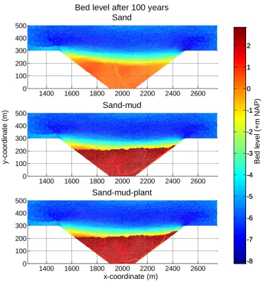
In figure 13 bed levels after 100 years of simulation are shown. The bed level in the upper figure is the result of simulating bed level changes by sand only. The middle figure shows the bed level with sand-mud interaction and the lowest figure shows the bed level of sand-mud interaction in combination with plants.

FIGURE 13 BED LEVEL AFTER 100 YEARS OF SIMULATING

The simulation with sand shows much lower bed levels than the other two simulations. The maximum bed level of the sand simulation is 0.76m. The maximum bed level of the simulation with sand-mud interaction is 2.87m and for the simulation including plants 2.83m. The

introduction of mud leads to significant higher bed levels. This effect is also visible in figure 14. 1400 1600 1800 2000 2200 2400 2600

0 100 200 300 400 500

Bed level after 100 years

Sand

1400 1600 1800 2000 2200 2400 2600 0 100 200 300 400 500

Sand-mud

The average bed level for the simulation with sand is significantly lower than the simulations with mud.

FIGURE 14 DEVELOPMENT AVERAGE BED LEVEL. THIS GRAPH ONLY CONSIDERS LOCATIONS WITH A BED LEVEL HIGHER THAN 0M IN THE END-SITUATION

The difference in bed level between a simulation with and without mud is explained by settling lag. Mud has a smaller particle size than sand and therefore it takes longer for mud to settle. The result is that mud can deposit particles on higher bed levels leading to a higher marsh. Settling lag also requires higher velocities to erode mud once settled. This effect is enhanced by cohesive properties of mud as when enough mud is available, it is able to trap sand and form a coherent mass.

Figure 14 also shows that after 100 years the simulations with mud are close to equilibrium as bed levels almost reach a constant value (which is below maximum spring tide). These lines fluctuate (especially at the beginning) from a large increase towards a smaller increase. These fluctuations are explained by the spring-neap cycle and the applied morphological acceleration factor of 100. When spring tides occur more sediments are deposited and higher bed levels are reached. For neap tides the opposite is true. The morphological acceleration factor enhances this effect. The simulation considering only sand still shows relative large bed level growth. To really determine when the sand simulation shows equilibrium conditions, simulation period has to be extended. This falls beyond the scope of this study.

Although maximum bed levels of the sand-mud and sand-mud-plant simulation are in the same order of magnitude, the bed pattern shows differences. The simulation with plants has more and smaller tidal creeks than the simulation without plants (see Table 5). When marsh is inundated, water is discharged through the creeks. The presence of plants cause velocities to decrease as water is discharged away from the marsh. Because flow velocities are reduced, more creeks arise to discharge all water away from the marsh platform (see also table 5).

0 10 20 30 40 50 60 70 80 90 100

0 0.5 1 1.5 2 2.5

Development average bed level

Time (years)

B

e

d

l

e

v

e

l

(m

N

A

P

)

TABLE 5 PERCENTAGE CREEKS AND AVERAGE DEPTH CREEKS AND BED LEVEL ON THE MARSH (BED LEVELS OF CREEKS ARE ECXCLUDED IN DETERMINING THE AVERAGE MARSH BED LEVEL)

Case % Creeks on

marsh

Average bed level creeks (m NAP)

Average bed level marsh (m NAP)

Average depth creeks (cm)

Number of tributaries

Sand-mud 10.5 1.54 2.34 80 8

Sand-mud-plant 12.6 1.50 2.29 79 12

Vegetation reduces erosion of tidal and fluvial channels (D’Alpaos et al., 2005). However, a study by Temmerman (2007) showed that this reduction of erosion is only a local effect. Dynamic vegetation patches have a larger scale off-site effect. They obstruct flow and therefore cause flow concentration and channel erosion between vegetation patches. This results in more channels. Figure 13 and table 5 show that the simulation with plants has more channels supporting the theory by Temmerman.

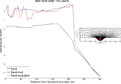
Figure 15 shows a cross-section after 100 years of modelling for a simulation with sand, sand-mud and sand-sand-mud-plants. The location where the cross-section is taken is indicated in the smaller subplot on the right side of the same figure with a red solid line. Again the large difference between a simulation with and without mud is clearly visible. Simulations with mud show much higher bed levels than the simulation with only sand. In the figure large fluctuations on the marsh are observed. This is because creeks cause differences in bed level. Taking a cross section 100 meters further would show different fluctuations. Figure 15 is therefore meant to show the general trend of different simulations.

FIGURE 15 CROSS-SECTION S OF THE SIMULATIONS WITH SAND, SAND-MUD AND SAND-MUD-PLANTS. IN THE RIGHT CORNER IS INDICATED WITH A RED SOLID LINE WHERE THE CROSS-SECTION IS TAKEN.

to its smaller grain size. Mud is therefore deposited further from the marsh edge (steep slope located around 200m from landward boundary in figure 15) on the marsh platform as here flow velocities are low enough for mud particles to settle. Vegetation and small water depths cause this decrease in velocity. Therefore the salt marsh edge consists of mainly sand resulting in the same slope in all simulations.

4.2 Plants

Figure 16 shows plant densities for the simulation with sand-mud and plants. On many locations on the marsh plants reach maximum plant density of 1200 stems/m2. Where plants do not establish tidal creeks are present. High inundation periods and velocities make it unfavourable for vegetation to establish in creeks. In addition there are some locations where plants did establish but were not able to reach maximum plant density. Most of these locations are adjacent to creeks. Because the simulation ends with a neap tide (relative low water levels), vegetation is able to establish next to the creeks.

FIGURE 16 PLANT DENSITIES FOR SAND-MUD-PLANT SIMULATION

Figure 17 shows the area development consisting of plants. Plants seem to move towards a dynamic equilibrium, and it looks like it is close to equilibrium after 100 years. The small fluctuations are again caused by the spring/neap cycle.

FIGURE 17 DEVELOPMENT OF AREA CONSISTING OF PLANTS

1400 1600 1800 2000 2200 2400 2600 0 100 200 300 400 500 x-coordinate (m) y-co o rd in a te ( m )

Plant densities for sand-mud-plant simulation

P la n t d e n si ti e s (st e m s/ m 2) 200 400 600 800 1000

0 10 20 30 40 50 60 70 80 90 100

0 1 2 3 4 5 6 7 8 9 10x 10

4 Plant area development

4.3 Mud content

In figure 18 the mud content for the simulation with and without plants is presented. The bed behaves cohesive when 30% of the bed consists of mud. Many locations reach this critical mud content. Nevertheless some locations on the marsh platform show a mud content around 0%. A part of these locations is clarified by the presence of tidal creeks. The flow velocities in tidal creeks withhold mud from settling. Furthermore, there are locations where no tidal creeks are present but still the mud content is around zero. This is explained by the bed becoming stable as no deposition or erosion occurs anymore. Due to vertical mixing, sand reaches the upper layer of the bed resulting in low mud percentages. This also explains why a decrease in mud content does not lead to a decrease in bed level.

FIGURE 18 MUD CONTENT AFTER 100 YEARS FOR SIMULATIONS WITH SAND-MUD AND SAND-MUD AND PLANTS

The outcome shows that mud content increases with distance from creeks. When flow enters the platform, it takes time for velocities to decrease in such a way that mud is able to settle, resulting in a sorting effect around the creeks from low mud percentages along the creek to high mud percentages further away from the creeks. This effect is indeed observed in figure 18 and corresponds with actual marshes.

4.4 Validation

Validation of results is limited in this thesis because an idealized situation is simulated. Seasonal variations like winter storms are not implemented in the model causing differences between actual and simulated development of salt marshes. Nevertheless, the growth rate, final elevation-, mud content- and vegetation pattern of the simulation are evaluated based on characteristics of Paulinaschor.

Paulinaschor shows sedimentation rates of 4 to 19 mm per year (Stikvoort et al., 2003). At the end of the 100 year simulation the sedimentation rates are close to these values (between 2 and 8 mm/year). However, because there is no real event in the model which causes erosion or sedimentation on bed levels higher than the maximum tide (storm events), sedimentation/erosion rates will eventually fluctuate around zero depending on the spring/neap cycle and morphological acceleration factor.

1400 1600 1800 2000 2200 2400 2600 0 100 200 300 400 500

Mud content after 100 years Sand-mud 10 20 30 40 50 60 70 80 90 Mu d p e rce n ta g e (% )

1400 1600 1800 2000 2200 2400 2600 0 100 200 300 400 500

Sand-mud + plants

FIGURE 19 CROSS-SECTION OF PAULINASCHOR

From AHN (Actueel Hoogtebestand Nederland) a cross-section is made from Paulinaschor (figure 19). The bed levels on the marsh platform correspond really well with the simulation with plants and sand-mud interaction (figure 15). Also the location of the marsh edge at 200 meters distance from the landward boundary is in correspondence with the simulation. A difference between the simulation and the actual cross-section is the height of the edge. In the simulation the marsh edge is about 4 meters high while on Paulinaschor the edge is about 2 meters and not as steep as in the simulation. The model was not able to reproduce a mud flat in front of the marsh resulting in a marsh edge of 4 meters. Causes for this difference could be the lack of waves and multiple sediment fractions in the model. Waves cause erosion of the marsh edge and multiple sediment fractions improve the sorting effect on the marsh (from large particles at the sea towards small particles at the landward boundary). Both processes result in a more gentle slope.

The marsh platform shows a slightly positive slope while in the simulation a negative slope occurs. However, both slopes are more or less flat.

Analysing soil characteristics of Paulinaschor, the soil mainly consists of mud, sandy mud and fine sand as can be seen in figure 36 in appendix 2. This graph shows higher probabilities of mud at the landward boundary than at the marsh edge which is in correspondence with literature (De Groot et al., 2011). This does not correspond with the simulations where mud content increases from landward boundary towards the edge. Because mud deposits first at the landward boundary, this part of the marsh is stable in an earlier stage than the marsh edge. Vertical mixing then causes sand to reach the upper layer decreasing the mud content.

Based on the validation of Paulinaschor the model adequately reproduces bed levels, plant pattern and location of the marsh edge. The model does not predict a mud flat which may be due to the lack of wind waves. Because this thesis concerns salt marsh development (and not mudflat) the model is assumed to be suitable for application towards the goal of this study, evaluating the contribution of different processes on salt marsh development.

5

SENSITIVITY ANALYSIS

In this chapter several processes are evaluated. The influence of tidal amplitude, boundary mud concentration, critical sedimentation shear stress, settling velocity for mud ,critical mud content and maximum bottom slope is checked. Before results are presented, each adaptation will be explained. When in this chapter “reference situation/simulation” is mentioned, the sand-mud-plant simulation is meant.

5.1 Process descriptions

5.1.1 Mud boundary condition of 100mg/L and 25 mg/L

In the initial situation the mud concentration is 50mg/L. These concentrations are imposed at the boundary of the morphological active zone meaning that tidal waves bring 50 mg/L of mud into the system. To evaluate the influence of mud availability, simulations are set-up which have a lower and higher mud concentration than the reference mud concentration. These concentrations are obtained from a paper by Verheyen et al. (2013). Verheyen determined the mud

concentration for the whole Western Scheldt. He found low concentrations of about 25mg/L at the seaward side of the Scheldt, while more land inward, at Land van Saeftinghe, concentrations of 100 mg/L were observed. Therefore these values are used.

5.1.2 Tidal amplitude

The influence of tidal amplitudes is assessed by increasing and decreasing the amplitude of different tidal components. The amplitudes are based on one-year data of the tide observed at Terneuzen. The average daily high amplitude is 2.35m NAP. A maximum daily amplitude is found to be 2.96m NAP and a minimum of 1.44 m NAP. These values are slightly exaggerated to evaluate extreme conditions, however it has to be taken into consideration that 100 years of extreme conditions is not very realistic. Still it provides a good insight of the influence of tidal amplitudes. The values of the M2-tide are based on values obtained from data, other tidal components are calculated by taking the ratio with the M2-tide. The amplitudes are presented in table 6. One month of low and high amplitudes are presented in figure 20.

TABLE 6 TIDAL AMPLITUDES FOR THE SIMULATIONS WITH HIGH AND LOW TIDE

Tidal component High Amplitudes (m NAP) Low amplitudes (m NAP)

M2

3.00

S2

1.04

MN4 0.015 0.005

FIGURE 20 SIMULATION WITH LOW AND HIGH AMPLITUDE

5.1.3 Continuous deposition

Some studies suggest to apply continuous deposition in order to obtain realistic results (Sanford & Halka, 1993; Winterwerp, 2007). This means that the critical sedimentation shear stress must be set very high in order for deposition to occur all the time. This is done in FINEL2D by applying a critical sedimentation shear stress of 1000 N/m2, while in the reference case the critical

sedimentation shear stress is 0.5 N/m2.

5.1.4 Low settling velocity of mud

In the reference situation a settling velocity for mud of 0.001 m/s is used. This value is obtained from a paper by Dam and Bliek (2013). A paper by Temmerman et al. (2003) suggests a ten times smaller settling velocity (0.0001 m/s). This value is implemented in the model.

5.1.5 Critical mud content of 20%

In the reference situation a critical mud content of 30% is applied. The critical mud content determines when the bed behaves cohesive. 30% of mud is suggested as the critical mud content in studies from Van Ledden (2003) and Mitchener and Torfs (1996). However, a study from Houwing (1999) found a critical mud content of 20% in the Dutch Wadden Sea. Although the Scheldt estuary is a different system, mud and sand should behave the same. Therefore it is interesting to analyse the effect of a critical mud content of 20%.

5.1.6 Maximum bottom slope of 0.5

In the simulation with sand-mud and sand-mud-plant a steep marsh edge arises. This edge is about 4 meters high. When analysing actual marshes, the slope should be more gentle. Therefore a simulation is done with a maximum bottom slope of 0.5. This means that when a bottom slope of 0.5 or less occurs in the simulation then erosion takes place according to an avalanche formulation.

Because now every process is described, results will be discussed.

5.2 Results

5.2.1 Bed level

contrast, bed levels are not really influenced by an increased mud concentration. The maximum bed level in the simulation with a concentration of 100 mg/L is 2.97 m NAP which is just slightly higher than the maximum bed level of the simulation with a concentration of 25 mg/L (2.79 m NAP). The simulation with low tidal amplitudes developed an error as the highest bed level is 7.32m NAP which is unrealistically higher than the rest of the marsh. Because flow velocities depend on water depth, the simulation with low tidal amplitudes has lower velocities than the simulation with high tidal amplitudes. The result is that in the simulation with low amplitudes deposition occurs on more locations leading to marsh expansion while the simulation with high amplitudes shows a relative small marsh.

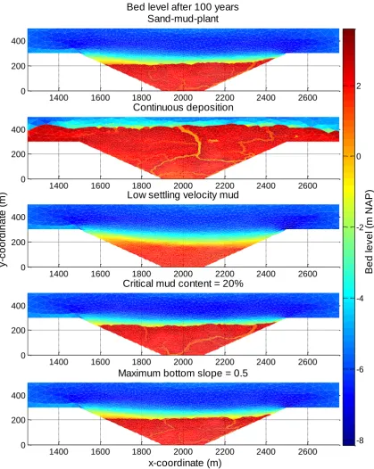
The simulation with continuous deposition expands more laterally than the reference simulation. Mud now also deposits on locations where shear stresses are higher than 0.5 N/m2 resulting in lateral marsh expansion. The creek occurring in the middle of the marsh in the continuous deposition simulation is much deeper than the rest of the creeks. This is caused by the fact that this creek has to empty most of the upper marsh after high tide.

For the simulation with a low settling velocity much lower bed levels arise in comparison to the other simulations. The settling velocity determines the deposition rate of mud. A smaller settling velocity implies that smaller flow velocities are required for mud to settle. Because boundary conditions do not change, flow velocities are the same as in the reference situation. Therefore less settlement of mud occurs. The result of the simulation with only sand and with a low settling velocity therefore look like each other as the bed in the situation with a low settling velocity also consists of mainly sand.

The simulation with a critical mud content of 20% shows a more laterally expanded marsh than the reference situation. When critical mud content is reached, the bed becomes cohesive. When cohesive, the bed is more difficult to erode. In this case the bed becomes cohesive in an earlier stage of the development resulting in less erosion. This leads to expansion of the marsh.

The difference between the simulation with a maximum bottom slope of 0.5 and the reference situation is small. When analysing a cross-section of both simulations can be seen that the simulation with a maximum bottom slope shows a slightly more gentle marsh edge (see figure 23 on page 38).

FIGURE 21 BED LEVELS AFTER 100 YEARS FOR SAND-MUD-PLANT,BOUNDARY MUD CONCENTRATIONS, AND TIDAL AMPLITUDES SIMULATIONS

1400 1600 1800 2000 2200 2400 2600

0 200 400

Bed level after 100 years

Sand-mud-plant

B

e

d

l

e

v

e

l

(m

N

A

P

)

1400 1600 1800 2000 2200 2400 2600

0 200 400

Boundary mud concentration = 100 mg/L

-8 -6 -4 -2 0 2 4

B

e

d

l

e

v

e

l

(m

N

A

P

)

1400 1600 1800 2000 2200 2400 2600

0 200 400

Boundary mud concentration = 25 mg/L

-8 -6 -4 -2 0 2 4

B

e

d

l

e

v

e

l

(m

N

A

P

)

1400 1600 1800 2000 2200 2400 2600

0 200 400

High tdal amplitude

-8 -6 -4 -2 0 2 4

B

e

d

l

e

v

e

l

(m

N

A

P

)

1400 1600 1800 2000 2200 2400 2600

0 200 400

Low tidal amplitude

FIGURE 22 BED LEVELS AFTER 100 YEARS FOR THE REFERENCE SIMULATION, CONTINUOUS DEPOSITION, LOW SETTLING VELOCITY FOR MUD, CRITICAL MUD CONTENT OF 20% AND A MAXIMUM BOTTOM SLOPE OF 0.5

1400 1600 1800 2000 2200 2400 2600

0 200 400

Bed level after 100 years

Sand-mud-plant

-8 -6 -4 -2 0 2

B

e

d

l

e

v

e

l

(m

N

A

P

)

1400 1600 1800 2000 2200 2400 2600

0 200 400

Continuous deposition

1400 1600 1800 2000 2200 2400 2600

0 200 400

Low settling velocity mud

1400 1600 1800 2000 2200 2400 2600

0 200 400

Critical mud content = 20%

1400 1600 1800 2000 2200 2400 2600

0 200 400

Maximum bottom slope = 0.5

y

-c

o

o

rd

in

a

te

(

m

)

FIGURE 23 CROSS-SECTION AT THE SAME LOCATION AS FIGURE 15 FOR THE REFERENCE SIMULATION AND A SIMULATION WITH A MAXIMUM BOTTOM SLOPE OF 0.5

Most simulations in figure 24 start with an average bed level of 0 m NAP at the beginning of the simulation. However, the simulations with continuous deposition and low tidal amplitudes start with a bed level smaller than 0 m NAP. This figure only considers bed levels which are above 0m NAP at the end of the simulation. Because the simulation with continuous deposition and low tidal amplitudes expand, bed levels which are initially below 0 m NAP are also accounted for. The lower bed levels, where eventually a marsh will develop, are significantly lower than 0m NAP so when deposition occurs on these locations, it really influences the graph as the average bed level starts to increase substantially. The simulation with continuous deposition even shows a decrease in average bed level at the beginning. This is explained by erosion which occurs in front of the marsh at the beginning of the simulation. During the simulation the marsh expands and average bed levels increase (see figure 25).

The highest bed levels are found in the simulation with high tidal amplitudes. The large amplitudes cause sediments to reach high locations. For the opposite reason the lowest bed levels are achieved in the simulation with low tidal amplitudes.

0 50 100 150 200 250 300

-5 -4 -3 -2 -1 0 1 2

Distance from landward boundary (m)

bed

lev

el

(m

+

N

AP)

Bed level after 100 years,

Reference

FIGURE 24 BED LEVEL DEVELOPMENT FOR THE DIFFERENT PROCESS SIMULATIONS

FIGURE 25 BED LEVEL DEVELOPMENT FOR SIMULATION WITH CONTINUOUS DEPOSITION. THE BLACK SOLID LINE IN THE SMALLER FIGURE REPRESENTS THE LOCATION OF THE CROSS-SECTION

0 10 20 30 40 50 60 70 80 90 100

-3 -2 -1 0 1 2 3

Development average bed level

Time (years)

Bed

lev

el

(m

N

AP)

Reference

Boundary mud concentration = 100 mg/L Boundary mud concentration = 25 mg/L High tidal amplitude

Table 7 shows results regarding creeks. The dimensions of creeks depend on different characteristics like discharged volume, bed level and expansion of the marsh. The two simulations which showed lateral expansion (low tidal amplitudes and continuous deposition) have a relative lower percentage creeks than other simulations. The expansions at the sides (see figure 26) do not require creeks for water to be discharged and therefore the marsh area is larger while the area consisting of creeks remains the same.

TABLE 7 RESULTS CREEKS

Case % Creeks

on marsh

Average bed level creeks (m NAP)

Average bed level marsh (m NAP)

Average depth creeks (cm)

Number of tributaries

Sand-mud-plant 12.6 1.50 2.29 79 12

High tidal amplitudes 8.0 2.69 3.45 76 5

Low tidal amplitudes 9.3 0.24 1.03 79 7

High mud concentration 10.5 1.58 2.42 85 9

Low mud concentration 10.2 1.17 2.02 85 9

Critical mud content 20% 12.5 1.41 2.31 90 12

Continuous deposition 9.2 1.14 2.15 1.01 13

Maximum bottom slope 13.7 1.57 2.29 72 13

FIGURE 26 LOCATIONS WHERE NO CREEKS DEVELOP

In the simulation with a low settling velocity for mud no real distinction between creeks and marsh platform is observed. The simulation with low settling velocities for mud requires a longer simulation period for the marsh to fully develop. However the question is whether settling velocity is high enough to develop a marsh with creeks.

5.2.2 Plants

In appendix 5 plant densities for all simulations are presented. These patterns are again

explained by the presence of creeks and inundation. More interesting is to analyse the total area consisting of plants (see figure 27). The simulations considering a high and low mud

concentration, critical mud content of 20%, high tidal amplitudes and a maximum bottom slope of 0.5 are close towards reaching dynamic equilibrium as their slope is almost flat at the end of the simulation. It is a dynamic equilibrium as plants can establish during neap tides while at spring tide vegetation decays.