Cross domain textual geocoding: the influence of domain specific training data

(1)

MASTER THESIS

Cross-domain textual geocoding:

influence of domain specific

training data

Mike C._Kolkman

Faculty of Electrical Engineering, Mathematics and Computer Science Human Media Interaction Research Group

Committee:

Dr. Djoerd_Hiemstra Dr. Mauricevan Keulen Dr. Dolf Trieschnigg Dr. Mena B.Habib

(2)

(3)

Abstract

Modern technology is more and more able to understand natural language. To do so, unstructured texts need to be analysed and structured. One such structuring method is geocoding, which is aimed at recognizing and disambiguating references to geographical locations in text. These locations can be countries and cities, but also streets and buildings, or even rivers and lakes. A word or phrase that refers to a location is called a toponym. Approaches to tackle the geocoding task mainly use natural language processing techniques and machine learning. The difficulty of the geocoding task is dependent of multiple aspects, one of which is the data domain. The domain of a text describes the type of the text, like its goal, degree of formality, and target audience. When texts come from two (or more) different domains, like a Twitter post and a news item, they are said to be cross-domain.

An analysis of baseline geocoding systems shows that identifying toponyms on cross-domain data has still room for improvement, as existing systems depend significantly on domain-specific metadata. Systems focused on Twitter data are often dependent on account information of the author and other Twitter specific metadata. This causes the performance of these systems to drop significantly when applied on news item data.

This thesis presents a geocoding system, called XD-Geocoder, aimed at robust cross-domain performance by using text-based and lookup list based features only. Such a lookup list is called a gazetteer and contains a vast amount of geographical locations and information about these locations. Features are built up using word shape, part-of-speech tags, dictionaries and gazetteers. The features are used to train SVM and CRF classifiers.

Both classifiers are trained and evaluated on three corpora from three domains: Twitter posts, news items and historical documents. These evaluations show Twitter data to be the best for training out of the tested data sets, because both classifiers show the best overall performance when trained on tweets. However, this good performance might also be caused by the relatively high toponym to word ratio in the used Twitter data.

(4)

(5)

List of Tables

2.1 Geonames statistics . . . 9

2.2 Corpora statistics . . . 10

4.1 Traditional performance metrics for baseline systems . . . 20

7.1 Macro average scores of SVM vs. CRF on the identification process . . . 36

7.2 Cross-domain macro average scores of the identification process grouped by training set . . . 37

7.3 Cross-domain macro average scores of the identification process grouped by test set 37 7.4 Precision, recall and F1 scores of three geocoding systems on the toponym identification and toponym disambiguation process . . . 39

A.1 Distance metrics for baseline systems . . . 44

C.1 Cross-domain PRECISION scores of the identification process grouped by training set . . . 49

C.2 Cross-domain RECALL scores of the identification process grouped by training set 50 C.3 Cross-domain F1 scores of the identification process grouped by training set . . . 50

C.4 Cross-domain PRECISION scores of the identification process grouped by test set 50 C.5 Cross-domain RECALL scores of the identification process grouped by test set . 51 C.6 Cross-domain F1 scores of the identification process grouped by test set . . . 51

(8)

(9)

List of Figures

2.1 Representation of an SVM including hyperplane examples . . . 7

4.1 Bar graph of theprecision of baseline geocoders per evaluation corpus . . . 21

4.2 Bar graph of therecall of baseline geocoders per evaluation corpus . . . 22

4.3 Bar graph of theF1-measure of baseline geocoders per evaluation corpus . . . 23

4.4 Bar graph of tradition IR metrics of the Oracle geocoder per evaluation corpus . 23 4.5 Bar graph of the mean error distance of baseline geocoders per evaluation corpus 24 7.1 Bar graph of the F1 score per test set . . . 38

B.1 Bar graph of the accuracy within a 10km radius of baseline geocoders per evaluation corpus . . . 46

(10)

(11)

1

Introduction to cross-domain geocoding

The amount of information available on the internet is vast and continuously growing. News sites post new items every few minutes, new blogs about all kinds of subjects arise every day and microblogging services like Twitter handle millions of posts per day. To handle, search and analyse all this language,named entity recognition is often an important first step. The goal of named entity recognition is to find all words or phrases, called entities, that refer to entities like a person, organization or location. Other entity types do exist, but are less common.

Once an entity is recognized, we need to determine which person, organization, location or other entity is exactly meant. This is done by finding the according entry in some database, called a knowledge base. The process of coupling a named entity word to its entry in a knowledge base is calledentity linking.

1.1 Geocoding

This research focuses on the spatial information in a text, i.e. descriptions of, or direct references to, geographical locations in a text.

Information about the location of a message or document can take multiple forms and be useful for various applications. Social media applications like Facebook and Twitter use the current location of devices to geotag the message. This way it is known from where a message was sent. Other location information that can be retrieved from messages are its spatial scope and spatial subject [28]. The spatial scope of a message or document is the area for which it is intended. E.g. the local newspaper is intended to be read by local residents and will thus contain mainly local news, whereas national newspapers will contain national and global news.

In this research the focus lies on the spatial subject of a message or document. The spatial subject of a message is the location a message, news item or document is about. Finding the spatial

(12)

subject in a text is a process which is called geocoding [18]. More specifically, geocoding is the process of identifying and disambiguating references to geographic locations, calledtoponyms. The process of geocoding can be divided in three sub-processes. In the toponym identification

step, words that refer to a location are identified. This can be considered a sub-problem of named entity recognition. Although the approach to toponym identification can be similar to that of named entity recognition, specific geographic information that is not available for other types of entities might help improve performance. Once toponyms are identified, candidate locations need to be found for each identified toponym. A process calledcandidate selection. This is often done by looking the toponym up in a gazetteer using lexical matching techniques. This step can be considered a pre-processing step for the last step oftoponym resolution. The toponym resolution process tries to select the location that the toponym is referring to. Information about the toponym, toponym context and candidate locations is used to select the most suitable candidate location. For a good geocoding performance, candidate selection should ensure a high recall. If the correct location is not among the candidates, the toponym resolution module will not be able to select the right location entity.

Building a geocoder is typically done using machine learning techniques like SVMs. As explained in more detail in chapter 3, most of the approaches described in literature use features which are highly dependent on the data source. Metadata like a geotag in Twitter is not available for data from news sites for example. In chapter 4, a data study is described which shows these geocoding systems’ performance declines significantly when evaluated on data from other sources than which the system is designed for. Some features that are used may not even be present in data from a different source. E.g. twitter messages may be geotagged, but most news items, magazine articles and other texts do not have any structured information of geographic nature. Geocoding systems that are NLP based are often more robust as they do not depend on metadata that is specific for one data source. Therefore, NLP systems might not score the best on data from any specific source, but do perform better on average than metadata based geocoders. This characteristic is advantageous when dealing with data from unknown sources.

1.2 Ambiguity

The main reason geocoding is a challenging task are the many ambiguities in natural language. These ambiguities exist in nearly every language and come in various types. In this section we discuss the types of ambiguity relevant to geocoding.

The type of ambiguity that is most relevant to toponym identification is called geo/non-geo ambiguity [20]. Geo/non-geo ambiguity states that many non-locations have the same name as a location. For example, “Washington” might refer to “Washington D.C.” in a recent news item, but is more likely to refer to “George Washington” in a historical context. Geo/non-geo ambiguity also infers locations that are named after common words or concepts. Examples include ”Love” (a small town in Mississippi) and a place called ”Dieren” in the Netherlands, which is also the

Dutch word for ”animals”. Handling this kind of ambiguity is essentially the task in the toponym identification step.

(13)

1.3. APPLICATIONS 3

Geo/geo ambiguity is the type of ambiguity directly related to toponym disambiguation [20]. It explains the ambiguity between two locations with the same or a similar name. For example, “Paris” is the capital of France, but there are around 35 places called “Paris” all over the world, most of them in the United States. Like Paris, a lot of famous places have other places named after them all over the world. A different kind ofgeo/geo ambiguity is the type where one location is contained in another, but they share the same name. For example, the city of “Luxembourg” lies within the district of “Luxembourg”, which itself lies within the country “Luxembourg”. To handle these kinds of ambiguity, a systems needs information including, but not limited to, the toponym context, the spatial scope of the text and the author’s location. Not all of these might be known for any arbitrary text.

1.3 Applications

Knowledge of the locations named in a text can be used in many applications. Various (research) fields might have an interest in automatically extracting locations from a text and plotting them on a map. This can for example be used for crime mapping. Automatically plotting crime locations from police reports or news items can help to identify crime hotspots, which can be used by criminology researchers, policy makers and city planners [19].

Visualizing (clusters of) locations can also be used for marketing purposes, to make marketing more targeted and therefore more effective. In a similar way, location information can help to supply users with location specific news and information. Location specific information can also help in question answering applications on questions like “Where can the Eiffel tower be found?”. If the entity “Eiffel tower” is extracted, the answer to the question can be retrieved with relative ease.

This research aims on antrending topic-like application for locations. Such an application would allow a user to identify focus locations of a group of texts. If geotag information is available, the scope of this focus can also be determined. In this context, the scope is the region that is interested in information about a certain location. For instance, the unstable situation in the middle east gets a global scope, whereas national football championships have a much smaller scope of interested people.

1.4 Research Questions

Chapter 4 describes an analysis of baseline geocoding system, which shows that most existing systems are capable of performing the geocoding task on data of a specific nature. However, when evaluated on data from a different domain, performance declines significantly. One could see such a system as domain dependent. Therefore, existing geocoding systems can not be considered robust to data domain changes and are not suitable to use on texts of an uncertain nature. A robust geocoding system should be able to handle these domain changes.

(14)

from the text. External data sources, like Wikipedia, can also be used for additional information, but were not utilized for this project.

For this research, we try to find an answer to the following questions.

1. How can a geocoder be made robust, so it performs similarly on data from various domains (e.g. social media, news items, etc.)?

2. Can a domain independent geocoder compete with domain dependent geocoders?

Of course it is unrealistic to expect a robust geocoder to achieve similar performance on a data set as a geocoder that was specifically designed for that data set. However, the goal of this project is to have the robust geocoder achieve reasonable performance compared to a specific geocoder. What should be considered as reasonable then depends on the performance of the specific geocoder and other things, like the amount of features, and the quality of those features, that can be extracted from the text. Short texts with bad grammar and many spelling errors are harder to geocode without the use of additional information, as they are less likely to follow standard language patterns.

(15)

2

Background

In this chapter background knowledge is given, which is required to fully understand the contents of this thesis. Note that some terms can be interpreted in different ways, so it is recommended to read this chapter even when you are familiar with the terms.

2.1 Named Entity Recognition

Named Entity Recognition (NER) is one of the major subtasks of information extraction. NER is aimed at the identification and classification of words and phrases that refer to certain entities, such as names of persons, organizations and locations [26]. Next to names, entities can also be dates, monetary values, etc. Example:

[ORG U.N.] official [PER Ekeus] heads for [LOC Baghdad]

This sentence contains three entities, with U.N. being an organization, Ekeus a person and

Baghdad a location.

NER is often used as a pre-processing step in natural language processing (NLP) systems, such as text classification and question answering. The performance of NER systems on traditional text data, like news items, achieves up to human-like performance. However, new types of data, like social media feeds, bring new challenges and require NER techniques to be adjusted and improved.

2.2 Entity Linking

Recognizing entities alone is insufficient in most use cases of NER. The entity linking task aims to map named-entities to a corresponding entry stored in a knowledge base (KB), for instance

(16)

Wikipedia. This knowledge base is often a large collection of entities (from one or more categories) and contains relevant information for each entry. The main goal of entity linking is to eliminate ambiguity. For instance,“president Bush”might refer to both George Bush Sr. and Jr. Linking the entity to the correct entry in the KB gets rid of this ambiguity. Furthermore, entity linking can be used to supply additional information about an entity in a text.

2.3 Machine Learning

Machine learning is a field of study based on statistics, that is about the construction of algorithms that can learn from data and can make predictions on new data.

One often used form of machine learning is supervised learning [16]. This form of machine learning works by presenting the system with example inputs and their desired outputs. The system should then “learn” a general rule that maps inputs to outputs. The system can then determine an output for new inputs, using the learned rule. How the system learns and applies this rule is dependent on the algorithm that is used. Other forms of machine learning exist, but are not relevant for understanding this thesis.

Supervised learning is often divided intoclassification andregression problems. For classification, the example inputs are divided into two or more classes. A machine learning system used for classification is called a classifier. After training on examples, the classifier should put new inputs into one of the classes. A well-known example of a classification problem is spam filtering, in which e-mails are assigned to the class ”spam” or ”not spam”.

In regression, the outputs are continuous, instead of discrete. Instead of assigning a class, some output value is assigned. E.g. a system that can predict house prices based on the properties of the house.

In this project, the task is to determine if a word is a toponym. This is similar to the spam filter, with in this case the classes being ”toponym” and ”not a toponym”. Therefore, the task at hand is considered a classification problem and is approached as such.

2.3.1 Feature extraction

Raw inputs are often not useful for machine learning algorithms. Therefore, features should first be extracted. Features are properties of the input in numerical form, so a machine learning algorithm can do calculations on them. The combination of features represents the observed input and is used as the direct input to the machine learning algorithm.

(17)

2.3. MACHINE LEARNING 7

2.3.2 Support Vector Machine

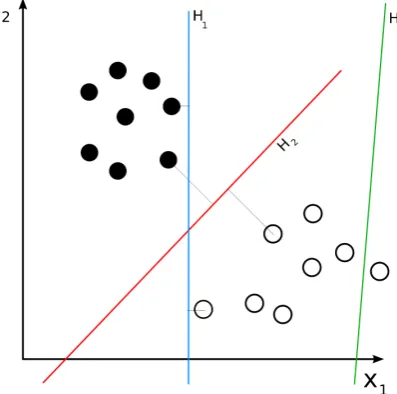
[image:17.595.182.381.186.383.2]

The support vector machine (SVM) is a supervised learning method, first proposed by Vapnik et al [6]. It can be thought of as a representation of the training examples as points in a space, as shown in figure 2.1. These points are clearly divided into two groups, the classes. The gap between the both groups should be as wide as possible for a clear division of the classes.

Figure 2.1: Representation of an SVM including hyperplane examples. Retrieved from http://commons.wikimedia.org/wiki/File:Svm separating hyperplanes.png, accessed 28-05-2015. Line H3 in figure 2.1 does not seperate the classes and H1 seperates the two classes with a small margin. Line H2 is the optimal division as it separates the two classes with maximum possible margin.

Note that the lines represent a hyperplane in a high dimension. For most problems the classes can not be separated linearly. Therefore, the SVM maps the original space into a higher dimensional space in which the separation is likely to be easier. The hyperplane with the maximum margin, represented in figure 2.1 by line H2, is called the maximum-margin hyperplane.

The examples closest to the separating line are called the support vectors, hence the name support vector machine. New examples are mapped into the same space, and classified based on the side of the line they fall on.

SVMs are originally designed for binary classification. Multi-class classification is done by reducing the multi-class problem into multiple binary classification problems. A common way of doing this is by using binary classifiers that make a separation between one class and the rest, called one-versus-all classification. If multiple classes are assigned by their respective binary classifier, the class with the highest margin on its binary classifier is assigned. Other methods exists, but are not relevant for this thesis.

(18)

2.3.3 Conditional Random Field

Conditional Random Fields (CRF) is a learning method focused on instance sequences, instead of single instances. Opposed to other sequencing methods, like hidden Markov models, CRFs find a probability distribution over label sequences given a particular observation sequence, instead of a joint distribution over both the label and observation sequences. This conditional approach makes that CRFs are less strict about the feature independence assumption that is required for other learning methods. Furthermore, CRFs do not suffer from the label bias problem, which can be caused by an unbalanced data distribution in other machine learning methods. The label bias problem occurs when a classifier performs very well on one class, at the cost of its performance on other classes. The disadvantage of CRFs is that most existing learning algorithms are slow, especially when the problem at hand requires a large number of input features. Because a CRF focuses on sequences, it is capable of processing sentences instead of single words. This makes that CRF approaches are often used for NLP tasks.

2.4 Labelling

To be able to train and evaluate a classifier, examples need to be labeled. Labeling can be done via various encodings [29]. For this research, both the BIO and IO encodings are used. In both cases, words get assigned a label. For the BIO encoding, the labels areBegin of toponym,

In-toponym andOut-of-toponym, whereBegin-of-toponym is assigned to all single-word toponyms and the first word in all multiple-word toponyms. In-toponmym is assigned to all other words in a multiple-word toponym andOut-of-toponym is assigned to all words not belonging to a toponym. This encoding is often used for training CRF models [27, 8, 1].

For the IO encoding, allBegin-of-toponym labels are replaced byIn-toponym labels. Because this encoding is binary, it is more suitable for classifiers like naive Bayes or Support Vector Machines (SVM).

2.5 Gazetteers

To be able to handle locations that are not in the training set, a gazetteer is often used. A gazetteer is an inventory of toponyms. These gazetteers often contain additional metadata about these locations, like its population size, comprehensive locations like country or state, and the locations surface size.

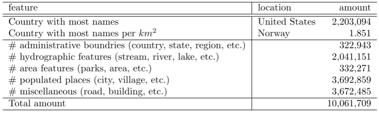
Multiple data sources exist for these gazetteers with varying detail. Which data source is used for a gazetteer is dependent on the project it is used for and the information detail this requires. The data source that will be used for this project is GeoNames1, as this is the most commonly used data source for global location gazetteers [11, 19, 20, 21, 32]. Furthermore, it is extensive and easy to use. This gazetteer contains over 15 million location names for over 10 million unique location entities. For most entities, the gazetteer contains a list of its names and aliases, its country code, various administration codes, population, elevation and timezone, as well as the geocoordinates of the center of that location.

(19)

2.6. CONTEXT DATA 9

feature location amount

Country with most names United States 2,203,094

Country with most names perkm2 _Norway _1.851

# administrative boundries (country, state, region, etc.) 322,943 # hydrographic features (stream, river, lake, etc.) 2,041,151

# area features (parks, area, etc.) 332,271

# populated places (city, village, etc.) 3,692,859

# miscellaneous (road, building, etc.) 3,672,485

[image:19.595.84.475.99.217.2]

Total amount 10,061,709

Table 2.1: Geonames statistics

2.6 Context data

To improve the resolution process, extra information of the toponym context can be used. Information about location bound concepts like buildings, and other associations to candidate locations can be very useful to make a better informed resolution. A good source for this data is Wikipedia, which contains pages of a vast amount of concepts and locations, of which many are geotagged [28, 32]. For this project, no context data was utilized.

2.7 Location types

Due to the corpora that are used, this system can only extract and resolve populated places, like countries, states, cities and municipalities. However, with more extensively annotated corpora, this might be extended to streets, buildings and other location dependent concepts like lakes and rivers. Evaluation of especially streets and rivers is hard, because of their oblong shape. Although this is a big issue in evaluating resolution systems, it is outside the scope of this project.

2.8 Gold standard corpora

For this research, four gold standard corpora from three domains are considered. These domains are microblog posts, news items and historical documents. In this section we describe all four corpora, by whom and how they were constructed and a listing of statistics about their build-up, like document count and token count. An overview of these statistics can be found in table 2.2.

2.8.1 GAT

(20)

For this research, a single tweet is considered to be a document. Hence, the maximum document size in the GAT corpus is 140 characters.

Note that the procedure of collecting tweets for this corpus makes this corpus very distant from a real-world case. Most tweets do not contain toponyms. Therefore, a system trained on the GAT corpus will very likely be biased and cause many false positives when run on a real-world set of tweets. Furthermore, by selecting the most ambiguous tweets, a toponym resolver is more likely to make mistakes.

Due to these selection choices by Zhang and Gelernter [34], this corpus can not be considered a good real-world representation of tweets. However, the GAT corpus still contains a lot of characteristics of microblogs, such as spelling errors, grammatical errors, and the use of special characters like hash tags. Therefore, I consider it to be useful for the cross-domain evaluation done in this research.

2.8.2 TR-CoNLL

TR-CoNLL is claimed to be the first corpus suitable for evaluating geocoding systems. It was built by Jochen Leidner as part of his PhD dissertation [18]. This corpus is a subset of the CoNLL2003 corpus, which was originally built for text classification tasks. The CoNll2003 corpus consists of texts from the Reuters news agency collected between 22 August 1996 and 31 august 1996. The TR-CoNll corpus is a subset of 946 documents from the CoNLL 2003 corpus, which was annotated with named entities. The resulting subset was then annotated with geocoordinates, resulting in a gold standard for geocoding containing 1903 annotated toponyms.

Most toponyms in TR-CoNLL (1685 out of 1903) refer to countries, with the other toponyms referring to states and cities. This makes TR-CoNLL very globally focused.

Due to this limitation, and because it is not freely available, I do not use the TR-CoNLL corpus for my evaluations. Instead, I use the more diverse, and freely available, LGL corpus, described in the next subsection. Because most existing systems described in the literature are evaluated using TR-CoNLL (among others), I do use reported performance statistics on the TR-CoNLL corpus in the baseline analysis reported in chapter 4.

GAT TRC LGL CWar

Data domain tweets news news historic

Document count 957 315 588 113

Token count 9872 68k 213k 25m

Average token/document ratio 10.3 216 363 221,239

Toponym count 818 1903 4793 85k

Average toponym/document ratio 0.85 6.04 8.15 752 Toponym/token ratio 0.0828 0.0279 0.0225 0.0034

Average ambiguity 16.5 13.7 3.7 31.5

[image:20.595.152.479.545.670.2]

Maximum ambiguity 432 857 382 231

(21)

2.8. GOLD STANDARD CORPORA 11

2.8.3 LGL

The few existing corpora, like TR-CoNLL, mainly contain news items from major newspapers. These news items are usually written for a broad geographic audience and is thus unsuitable for evaluating systems on smaller location entities. Therefore, Lieberman created the Local-Global Lexicon (LGL) corpus [20]. This corpus consists of 588 news items from a total of 78 smaller news sources originating from all over the world. All news items are in English and were collected in the months February and March of 2009. After collecting and selecting the news items, they were manually annotated, including references to the Geonames gazetteer. Opposed to corpora like TR-CoNLL, in which most toponyms refer to countries, most toponyms in LGL refer to villages and cities. Therefore, LGL is more suited for evaluating geocoding systems on a local level.

2.8.4 CWar

The Perseus Civil War and 19th Century American Collection (CWar) corpus2 _{is a data set}

containing 341 books mainly written about and during the American Civil War. Due to the historical content in this data set, it brings new challenges for natural language processing tasks like entity recognition and entity linking.

The CWar corpus is toponym annotated by Sperious et al. through a semi-automated process [32]. First, a named entity recognizer identified toponyms, after which coordinates were assigned using simple rules. These annotation were then corrected by hand. Due to this process, the CWar is relatively big. However, it also means the corpus is not very reliable. The manual corrections make that the corpus is fairly accurate, but the limitation of the used entity recognizer makes that the recall is fairly low. Therefore, correct classifications might be considered as false positives, due to the limitations of the corpus.

Although this will be a big influence on evaluation results, I still use this corpus for my evaluations. To my knowledge, it is the only toponym annotated corpus with historical content. Because the choice in toponym annotated corpora on different domains is limited, I choose to accept the limitations of this corpus.

(22)

(23)

3

Related work

In this section, related work on entity linking in general, and Twitter entity linking, and toponym resolution in particular is reviewed. Furthermore, work on context expansion is addressed.

3.1 Entity linking

Linking entities to some knowledge base can be regarded as providing unstructured data with semantics [24]. A simple, but often used approach is to perform lexical matching between (parts of) the text and concepts from the knowledge base [2, 31]. Although lexical matching is a good start for entity linking, it is unable to deal with ambiguity.

Handling this ambiguity is called (Named) Entity Disambiguation. Many approaches for this have been proposed, nearly all of which use the entity context to gain information about the entity [10, 25, 35]. These methods turn out to work well on larger documents with sufficient context, but are less effective on smaller documents like microblog posts.

3.2 Geocoding

Geocoding is a special form of entity linking. The first distinction is that it is specifically focussed on geographical entities. Secondly it can link entities to geo-coordinates, instead of a knowledge base. This makes that toponym resolution systems can be evaluated independent of the knowledge base that is used. A downside to this is the decreased reliability of evaluation results, because knowledge bases might have slightly different coordinates for the same location. Furthermore, most locations can be considered to be an area, and not just one coordinate. For buildings and even small cities this might not be a problem, but for larger entities like states and countries, a single coordinate does not supply sufficient information to identify a unique location entity.

(24)

Quercini et al. [28] propose a toponym resolution method, to improve the search for news feeds, based on the users location and the spatial focus, and spatial subject of the news source. To determine the spatial subject of a document, they first resolve the toponyms in that document. They build their toponym resolution system around the notion that each location has a local lexicon of spatially related concepts, i.e. concepts that have a strong association with that location. For example, the local lexicon of Enschede contains concepts likeFC Twente,University of Twente

andOude markt. Quercini et al. use Wikipedia to find spatially related concepts to their candidate locations. They first build a set of spatially related concepts for each spatial concept in Wikipedia. Secondly, they propose a metric for the spatial relatedness between concepts, and only keep the 20 most related concepts to that location. In the toponym resolution process, they then determine the likeliness of a candidate location, based on the amount of concepts that occur in the document, as well as the local lexicon of that candidate location.

WISTR is the best reported system by Speriosu et al. [32]. It is based on a similar notion as the previous mentioned system by Quercini et al, i.e. that documents are likely to contain concepts that are spatially related to the toponym that is being processed. In their paper, Speriosu et al. propose various methods to leverage this notion, of which a system called WISTR is the best performing. WISTR assumes that spatially related concepts can be found within a 10km radius of the candidate location, and that each mention of a single toponym in a document refers to the same location. The system looks up each n-gram, with various n, in a geotagged version of Wikipedia. If a concept’s coordinates lie within the mentioned 10km radius, that concept is considered to be related to the toponym. From these related concepts, features are extracted to train logistic regression classifiers. WISTR finally chooses the candidate location for which the classifier returns the highest probability.

The system that is proposed in this research will try to apply the concepts used by Quercini et al. and Speriosu et al. to documents with less context. Because the before mentioned systems rely heavily on the availability of sufficient context, in the following we describe some researches that address the issue of limited context in microblogs.

3.3 Microblog entity linking

Performing entity linking on microblogs, like Twitter, can increase search performance significantly. However, due to the fuzzy nature of microblogs, entity linking on microblog content is hard [24]. The limited entity context provides little information to base decisions on. Take for example the following tweet from an Australian national debate in 2011:

”No excuse for floods tax, says Abbott”

Without any knowledge about what the floods tax is, or that the poster is Australian, it is not clear thatAbbott is actuallyTony Abbott, the Prime Minister of Australia. Also, the often used knowledge base Wikipedia, contains over 500 pages containing the wordAbbott, including the spelling variationAbbot, which is a religious title. This shows that having only limited context, makes disambiguation a hard task [9].

(25)

3.4. GEOCODING IMPROVEMENT 15

concept is manually annotated as being relevant or not to the tweet. They use this manually annotated set as a training set for their classifier. In their paper, it is specifically noted that the first step of finding candidate concepts might be omitted, but is very important, because it reduces the number of feature vectors that need to be created, which significantly decreases the runtime. The features that are extracted are mainly focussed on the hyperlinking structure of Wikipedia. Features include, but are not limited to, the number of Wikipedia articles linking to a concept page, the number of Wikipedia articles that are being linked to by the concept page, and the number of Wikipedia categories that are associated with the concept. Furthermore, they leverage Twitter specific properties to a message, like hashtags, by using boolean features, e.g. does the tweet contain the title of the concept page. The system by Meij et al. has some similarities to the method proposed in the current research. However, where Meij et al. link complete tweets to concepts, the current research is aimed on the linking of toponyms, which is a lot more error prone. Furthermore, the current research is aimed at linking toponyms, which makes it possible to use specific characteristics like the distance between the candidate location and the concept location.

3.4 Geocoding improvement

The issue of limited context in microblog messages can be dealt with by expanding this context. Adding more context to the tweet or using information about a candidate location as context can increase performance significantly [9].

Guo et al. propose a method to link entities in tweets to Wikipedia concepts. They base their method on the notion that microblogs are:

short each message consists of at most 140 characters.

fresh tweets might be about a concept or event, that is not yet included in the knowledge base. informal tweets commonly contain acronyms and spoke language writing style.

As mentioned before in the current proposal, this means microblog posts provide little context. To overcome this issue, Guo et al. leverage another property of microblogs:

redundancy microblog posts about the same subject tend to contain similar information in different expressions.

(26)

(27)

4

Performance analysis of baseline geocoding

systems

This chapter describes a small baseline study, to find the difficulties in the various data sets and to analyse the strengths and weaknesses of some simple baseline approaches.

4.1 Setup

In this study, I look to find the difficulties in geocoding on corpora from different domains. To do this, I set up an experiment with the corpora GAT, TRC and CWar from the microblog, news and historical domain respectively. Six systems with various complexity are run and evaluated on these sets. Five of the six systems come from theFieldspring project by Speriosu [32], who also uses these systems as his baseline. One system is calledCarnegie, and is made by Zhang and Gelernter [34], which they evaluated using their GAT corpus. This last system can be seen as a domain dependent geocoder, as it makes extensive use of the metadata provided with Twitter messages.

All Fieldspring systems use the same named entity recognizer for toponym identification, of which the Stanford POS tagger is the main component.

Oracle The oracle always chooses the candidate location, closest to the gold standard location. If the annotation was done using the same gazetteer as used by the system, this means the score of the oracle resolver will be 100%.

Random Randomly choose one of the candidate locations

Population Always chooses the candidate location with the biggest population

BMD Basic Minimum Distance resolver. This resolver chooses those candidates that minimize the overall distance between the resolved locations. This is based on the premise that

(28)

toponyms in a text are often spatially related, and thus their mutual distance is often relatively small.

SPIDER SPIDER (Spatial Prominence via Iterative Distance Evaluation and Reweighting) is a variation to BMD. It tries to accomplish the same goal, meaning it will try to minimize the overall distance between the chosen locations. However, SPIDER uses a different algorithm, which first tries to find clusters of locations. Per iteration, it assigns weights to each candidate location based on its distance to the candidate locations of other toponyms in the same document and the previous weight. According to Speriosu and Baldridge [32], these weights converge on average after 10 iterations. The candidates with the highest weights after these 10 iterations then get selected.

Carnegie This system extracts features from the metadata of the tweet and uses these to train SVMs. This system also uses a different NER system for the identification step, which obtains a far better score than the Stanford NER which is used by the Fieldspring resolvers. The oracle resolver was included, because it gives the isolated performance of the toponym identification, due to the 100% resolving score. This way, we get an idea of the influence of the identification step on the complete geocoding process. The random resolver can be seen as a worst case performance, which gives an indication of the value of the performance of the other resolvers, as well as the difference in resolving difficulty of the three corpora.

Note that the strengths of BMD and SPIDER are achieved through the relation between multiple toponyms in a single document. For news items, this premise might be very useful. However, on a domain like microblog messages, the character limit allows for little toponym co-occurence possibilities. Therefore, it is likely these systems will score far less on the Twitter data in the GAT corpus.

Evaluation of a geocoder can be done in two fashions. Gold toponym evaluations use the annotation from the evaluation corpus for the identification step. This means the performance of the resolution step gets evaluated in isolation. However, because the annotated toponyms are used for the identification step, this means that the total number of disambiguated toponyms will always be equal to the total number of annotated toponyms. From this and the definitions of precision and recall above follows that precision equals recall for these evaluations. Gold toponym evaluations are denoted withGT in the tables and figures.

NER evaluations use Named Entity Recognition systems to do the identification step of the geocoding process. Note that all baseline resolvers, with exception of the Carnegie system, use the same Named Entity Recognizer for their NER evaluation. This means they all have the exact same score for the identification process. NER evaluations are denoted withNER in the tables and figures.

The systems are evaluated using traditional information retrieval metrics precision, recall and F-measure. The following definitions are used for these metrics.

Precision The number of correctly disambiguated toponyms, divided by the total number of disambiguated toponyms.

Recall The number of correctly disambiguated toponyms, divided by the total number of annotated toponyms.

F-measure The harmonic mean of precision and recall, defined as 2_precision∗precision₊∗_recallrecall.

(29)

4.2. RESULTS 19

the results for real-world applications where geographical accuracy is less important. For instance, when looking at a global map, resolving the correct country might be good enough to make an application useful, whereas a map of a single country requires cities to be correctly resolved as well.

Distance metrics only reflect the disambiguation performance. Unidentified toponym simply are not considered for these metrics. Therefore, there is no analogue for recall among the distance metrics. The distance metrics that are reported are the following:

Minimum error distance A high minimum error distance reflects a poor disambiguation performance. Since a single exact match sets this metric to 0.0, it is not very useful in most cases.

Maximum error distance If the maximum distance error is small, it shows the disambiguation system is very accurate. On the contrary, this value indicates little about the system performance when it is big, as it might be caused by an outlier. Chances that no such outlier errors are made, are really small. Thus, this metric says little about system performance in most cases.

Mean error distance The distance between the resolved coordinate and the ground truth is measured for all toponyms and then averaged. The main problem with this metric is the big influence of a couple of large errors on the average error. Therefore, a high mean error distance often goes hand in hand with a high maximum error distance.

Median error distance To pass the problem of the mean distance error, the median distance error is often reported. This metric emphasizes that small errors are acceptable.

Accuracy within x km This metric is similar to the precision metric, however it takes a correctness radiusx, in which errors are accepted. Values for x∈ {10,50,100,161} are reported.

For this comparison study, the results on the TR-CoNLL corpus were retrieved from literature, as this corpus is not freely available. Also, all results of the Carnegie system were retrieved from literature, as the system itself is not published.

4.2 Results

In this section the results of the evaluations are described.

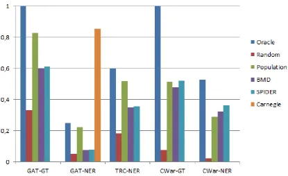
First, I discuss the performance differences between the baseline systems overall using the traditional information retrieval metrics. Secondly, I discuss these differences using some distance metrics. Finally, the differences of the system performances between the various domains are discussed, using both traditional IR metrics and distance metrics.

(30)

GAT-GT GAT-NER TRC-NER CWar-GT CWar-NER

Precision 1.0 0.672 0.826 1.0 0.136

Oracle Recall 1.0 0.249 0.599 1.0 0.527

F1 1.0 0.364 0.694 1.0 0.216

time (min) 0.06 0.06 NA 0.84 0.91

Precision 0.332 0.140 0.251 0.074 0.005

Random Recall 0.332 0.052 0.182 0.074 0.021

F1 0.332 0.076 0.211 0.074 0.009

time (min) 0.05 0.05 NA 0.80 0.89

Precision 0.827 0.601 0.716 0.515 0.075

Population Recall 0.828 0.223 0.519 0.515 0.290

F1 0.828 0.325 0.602 0.515 0.119

time (min) 0.06 0.05 NA 0.85 0.85

Precision 0.603 0.205 0.479 0.478 0.083

BMD Recall 0.603 0.076 0.347 0.478 0.321

F1 0.603 0.110 0.402 0.478 0.132

time (min) 0.06 0.06 NA 2.45 11.46

Precision 0.613 0.212 0.491 0.522 0.094

SPIDER Recall 0.613 0.079 0.356 0.522 0.363

F1 0.613 0.115 0.413 0.522 0.149

time (min) 0.07 0.06 NA 7.78 27.72

Precision NA 0.850 NA NA NA

Carnegie Recall NA 0.855 NA NA NA

[image:30.595.115.520.100.396.2]

F1 NA 0.852 NA NA NA

Table 4.1: Traditional performance metrics for baseline systems on 3 different corpora (NER and GT evaluations). Note that in this table the TRC-GT results are omitted, as they are not available.

with the SPIDER system on the CWar corpus are small ( .05), whereas the population system outperforms the SPIDER and BMD systems greatly ( .2) on the other corpora.

The performance differences in favour of the SPIDER system to the BMD system are very small (max .044) for all metrics on all corpora. Note that this small gain in performance comes at a

relatively high computational cost compared to the BMD system.

As the Oracle system achieves a 100% score on the resolving step, the NER scores reflect the performance of the named entity recognizer. Results on all 3 corpora show that the recognizer used in the Fieldspring systems has a lot of room for improvement, with a maximum F1-score of .694 on the TRC corpus. Furthermore, its F1-score of .364 on the GAT corpus show it is far from robust for cross-domain purposes. Figure 4.4 shows that the NER precision is higher than its recall on both the GAT and TRC corpus. For the Cwar corpus, precision is very low with the recall being reasonable compared to the recall on the other corpora.

Note that for the mean error distance values in figure 4.5, the smaller the value the better the performance. Also, the distance metric table does not contain the Carnegie system, as these metrics were not reported by Zhang and Gelernter [34].

(31)

[image:31.595.78.478.97.345.2]

4.3. DISCUSSION 21

Figure 4.1: Bar graph of theprecision of baseline geocoders per evaluation corpus

each combination, which says little about the overall performance of the system. Looking at the differences in mean error distance of the resolvers, we see that the population system scores well on both the GAT and TRC corpus compared to the BMD and SPIDER systems. For the CWar corpus we see similar differences, however this time in favour of the BMD and SPIDER systems. The median error distance shows a similar pattern. Notable is the relatively high median error distance of the BMD and SPIDER systems on the GAT-NER corpus.

For the accuracy measurements, we would expect a larger correctness radius to improve the accuracy value, as larger error distances are accepted. On the GAT corpus this hypothesis is confirmed with an increase up to .38. However, this increase in accuracy is minimal on the CWar corpus.

4.3 Discussion

The robustness of the population resolver shows population data is a valuable feature for resolving toponyms. The performance of the population resolver on the GAT-GT corpus shows that locations mentioned on Twitter are often large populated places. This might be due to the fact that big cities host more events and are therefore a more interesting topic for Twitter users. On the CWar corpus, population data turns out to be less useful. This is probably due to the fact this war was fought mostly on open fields, in woods and in small villages, of which some might not even exist anymore. Therefore, larger populated places are mentioned less in this corpus, compared to more recent articles.

(32)

[image:32.595.113.529.98.352.2]

Figure 4.2: Bar graph of the recall of baseline geocoders per evaluation corpus

(33)

[image:33.595.79.495.104.359.2]

4.3. DISCUSSION 23

Figure 4.3: Bar graph of theF1-measure of baseline geocoders per evaluation corpus

[image:33.595.71.492.408.657.2]

(34)

[image:34.595.113.546.199.513.2]

(35)

5

Feature design

5.1 Methodology

The most important goal of this system is that it has to be independent of a specific data source. Therefore, the features used for this system are chosen based on their independence of a specific data domain. Following multiple researches [30], the features are divided into multiple groups. In these researches, the list of groups often contains some base group, a group of gazetteer features, a group of dictionary features, a group with bag-of-word features and a group of other features specific to the task at hand. Because this last group is specific to the task, it is also specific to a data domain, and therefore less useful in this research.

5.2 Feature descriptions

Features are extracted per token. One feature vector thus contains the features of a single token, although it might also contain context token features. In the following subsections we describe the feature groups and the features they contain.

5.2.1 Base features

The base group of the built system is focused on lexical and part of speech features. The first features are focused on capitalization, as this is an important feature for identifying named entities:

IsUppercase binary feature that denotes if the token is capitalized. Capitalization is an important indicator of named entities in English. For other languages like German, this feature is less useful, because all nouns are capitalized in German.

(36)

IsAllCaps binary feature that denotes if the token is in all caps. Words that are fully capitalized are often special words or acronyms, and are less likely to be a toponym.

HasPrefix(j) binary features that denote if the token has prefix j. The set of prefixes consists of the most common prefixes for toponyms in English. This set is retrieved from Wikipedia1. This list could be expanded with relevant prefixes for other countries if necessary. For this project, it was limited to the English toponymy.

HasSuffix(j) analogously to HasPrefix(j), but for suffixes.

PartOfSpeechTag(k,t) dummy coded feature that denotes if token k has part-of-speech tag t according to the Stanford PoStagger, where k is the previous token, current token or next token. This would thus lead to 3 PartOfSpeechTag features per feature vector. In most cases, a toponym is a noun. Furthermore, it is likely for a preceding word to be a preposition (in, to, towards, from, etc.).

5.2.2 Dictionary features

Although these features are very powerful in finding named entities, only the prefix and suffix features provide specific information about toponyms. Therefore, more information related to toponyms is required. In the group with dictionary features we use the occurrences of toponyms in the training set:

WordIndex The index of the token in de dictionary, which consists of all words in the training set.

WordFrequency The frequency the token is seen in the training set.

IsToponymFrequency The frequency at which the token is seen as a toponym in the training set.

IsToponymFraction IsToponymFrequency divided by WordFrequency. If the WordFrequency is zero, IsToponymFraction will take the value 0.5. This is because a value of 0 would imply the word is never a toponym, whereas a value of 1 would imply the word is always a toponym. Neither is the case, as the word has never been seen in the training set. This feature is very powerful in distinguishing geo/non-geo ambiguity. Words that are rarely seen as toponym in the training data, are less likely to be a toponym.

IsInitialInToponymFrequency The frequency at which the token is seen as the first token in a toponym in the training set.

IsInitialInToponymFraction IsInitialInToponymFrequency divided by WordFrequency. If the WordFrequency is zero, IsInitialInToponymFraction will take the value 0.5. This is because a value of 0 would imply the word is never a toponym, whereas a value of 1 would imply the word is always a toponym. Neither is the case, as the word has never been seen in the training set.

IsPartOfToponymFrequency The frequency at which the token is seen as a partial token of a toponym in the training set.

(37)

5.2. FEATURE DESCRIPTIONS 27

a value of 0 would imply the word is never a toponym, whereas a value of 1 would imply the word is always a toponym. Neither is the case, as the word has never been seen in the training set. This feature is essential for multi-word toponyms, like “United States of America”.

UppercaseFrequency The frequency at which the token is seen uppercased in the training set. UppercaseFraction UppercaseFrequency divided by WordFrequency. If the WordFrequency is

zero, UppercaseFraction will take the value 0.5. This is because a value of 0 would imply the word is never a toponym, whereas a value of 1 would imply the word is always a toponym. Neither is the case, as the word has never been seen in the training set. A word that is usually lowercased (low uppercase fraction), is more likely to be a named entity when seen uppercased.

5.2.3 Gazetteer features

The dictionary features give the system more information about toponyms and specifically the feature ToponymFraction intuitively seems a good indicator of a toponym. However, toponyms that are never mentioned in the training set are left out by this feature. Therefore, the group of gazetteer features is added, to provide real-word information:

InitialInGazetteer(k) This binary feature denotes if token k is the initial word in a toponym in the gazetteer, where k is the previous token, current token or next token.

PartiallyInGazetteer(k) This binary feature denotes if token k is part of a toponym in the gazetteer, where k is the previous token, current token or next token.

FullyInGazetteer(k) This binary feature denotes if token k is a toponym in the gazetteer, where k is the previous token, current token or next token.

(38)

(39)

6

XD-Geocoder: System implementation

To evaluate the influence of the data domain on the performance of a geocoder, I built a cross-domain geocoder, which I named the XD-Geocoder. The system was built in Java. In this chapter, the structure, implementation details and used libraries of the XD-Geocoder are described. The source code can be found at GitHub1.

The system was built with the intention to accommodate any corpus format. Furthermore, it had to be easy to switch out the used machine learning library for any arbitrary machine learning library. To accomplish this, the system is divided into five modules. These modules and its implementations are described in this section.

6.1 I/O

The I/O module contains the readers and writers for the various data objects. This module is divided in a part for the corpora, and a part for gazetteers. The implementation for the

GazetteerReaderinterface is limited to the Geonames gazetteer, whereas there are implementations for theCorpusReaderinterface for the GAT corpus (twitter data), LGL corpus (news items) and CWar corpus (historical texts). Other implementations of the CorpusReaderinterface were also built, but not used for this research.

TheGazetteerReaderis designed to returnLocationobjects. For the Geonames gazetteer, these locations are read from theallCountries package, which can be downloaded from the Geonames website2. These locations were then all saved into memory through aLocationGazetteer object. Because the allCountries package is rather large, the XD-Geocoder requires at least 8 GB of main memory. The gazetteer is accessed frequently, so using an external database would make the system unnecessarily slow.

1_{https://github.com/mkolkman/XD-Geocoder} 2_{http://download.geonames.org/export/dump/}

(40)

TheCorpusReaderimplementations returnDocumentobjects. Documentobjects can be tweets, news articles or book chapters. All contain aString text, and a list of Toponymobjects. How theseDocumentobjects are loaded depends on the data source. The data sources used for this research were either CSV or XML files and were thus relatively easy to parse. TheCorpusReader

is to be used as the first part of the classifier pipeline, which is described in more detail in the rest of this chapter.

6.2 Preprocessing

Once the gazetteer and corpus are loaded, the documents need additional preprocessing before the features can be extracted. Preprocessing is done using apipeline-like architecture. This pipeline is implemented through aWord iterator. All classes in the pipeline implement this iterator and accept aWorditerator as input.

For now, the pipeline only contains three components, which are described in the following. Other preprocessing components that may be needed for the extraction of other features, can easily be added by implementing theWorditerator.

6.2.1 WordTokenizer

The first component of the pipeline is theWordTokenizer. As it is the first component of the pipeline, it is the only part of the pipeline that does not accept aWorditerator as input. Instead, theWordTokenizerrequires a String text. TheWordTokenizerthen splits this text up into tokens. For this implementation I used the Stanford PTBTokenizer, developed by Christopher Manning et al [22].

Once the texts are tokenized, we have our first instance of aWord iterator. However, these words are only plain text and their position in the text. To extract more interesting features, some more preprocessing is required.

6.2.2 POS tagger

The part-of-speech (POS) tagger is required for the extraction of the POS features. For the POS-tagger in XD-Geocoder, the Stanford Maximum Entropy tagger [22] is used based on the Left3Words model for English. This tagger assigns one of the tagsDETERMINER,PREPOSITION,

ADJECTIVE, NOUN, ADVERB, INTERJECTION, VERB, CONJUNCTION, PRONOUNor OTHER to the word. As explained in section 5, especially the tagNOUN is a good indicator a word might be part of a toponym.

(41)

6.3. TOPONYM IDENTIFICATION: TRAINERS AND CLASSIFIERS 31

6.2.3 Labeler

The labeler assigns labels to the words following the BIO or IO encoding, which are described in more detail in section 2.4. Labels are determined from the gold standard corpus for training and evaluation of the classifiers. For real-world applications, a labeler can be build, which takes a

Classifier object and uses this classifier to determine the assigned labels.

6.2.4 Feature extraction

Each feature value is represented as aFeaturemodel which accepts aWordobject, and calculates a boolean or float value. Thus the system contains classes HasPartOfSpeechTag, HasPrefix,

IsCapitalized, etc.

The FeatureExtractor creates these Feature models for each Word and adds them to a

FeatureVector. Thus, a text is transformed into a sequence of FeatureVectorobjects.

6.3 Toponym identification: trainers and classifiers

The extractedFeatureVectorobjects are wrapped intoLearningInstanceobjects, which also contain the accordingWordand Labelobject.

The aforementioned process results in a sequence ofLearningInstanceobjects. TheseLearningInstances are then used as input for aClassifierTrainerobject. This object implements atrainfunction,

which returns aClassifier object.

6.3.1 Mallet

The used classifiers are built using the Machine Learning for Language Toolkit (Mallet). This is a Java-based package mainly focused on statistical NLP, document classification, information extraction, and other machine learning applications for natural language text. Mallet was created at the University of Massachusetts by Andrew McCallum [23].

For this research, I used the Maximum Entropy and CRF classifier contained in the Mallet package. Furthermore, I used the SVM implementation from the LibSVM package created by Chang et al [3].

6.3.2 Support Vector Machine classifier

Because Mallet does not contain an SVM classifier, I used the Mallet wrapper for LibSVM [3] by Syeed Ibn Faiz of the University of Western Ontario3. This classifier is highly customizable. Although implementing the SVM classifier is simple, customizing and tuning of the SVM kernel and its training parameters is a time consuming job.

For the tuning of the SVM kernel I followed a procedure mostly inspired by the guide for LibSVM by Hsu et al [12]. First, feature extraction was performed. SVMs tend to perform better when

(42)

feature values are normalized [13]. Because theXD-Geocoder uses mainly boolean features, scaling was not performed for this project. As recommended in the guide by Hsu et al [12], the first kernel that was used is a Radial Basis Function (RBF) kernel.

Handling unbalanced data

The first results using this kernel were unsatisfactory, because of the unbalanced nature of the data (see chapter 2). The unbalance in the data resulted in a 100% classification to theOut-of-toponym

class, which results in a macro F1 performance of 0.97. This is caused by the fact that, because of the relative small size of the classes, errors in theBegin-of-toponym and In-toponymclasses have limited effect on the system’s macro performance.

Literature suggests three possible solutions to this problem [14]. The first solution is random undersampling [15], which aims to balance class distribution by randomly eliminating majority class examples. This way, the difference between the class sizes is limited and the classifier should lose its bias towards the majority class. The major drawback of the undersampling method is the loss of (most of the) potentially useful majority class examples. The counterpart of undersampling is oversampling, which aims to balance class distribution by randomly duplicating minority class examples. Although this method does not lead to the loss of potentially useful examples, multiple papers state that oversampling increases the risk of overfitting significantly [4]. The last, and in this research used, approach is based on cost-sensitive learning [7]. This approach assigns fixed cost weights to each class in order to equalize misclassification costs between classes. The weights are chosen based on the proportions of the class examples in the training set using the formula Wi =

|B|+|I|+|O|

|i| , where Wi is the weight assigned to class i, with i∈ {B, I, O}. B is the

Begin of toponym class,I theIn toponym class andO theOut of toponym class.

First experiments showed that assigning class cost weights has the desired effect, as the classifier lost its bias towards the majority class. Experiments with tuning the class cost weights using a grid search with various deviations showed no positive effects on the systems performance. Therefore, the class cost weights are assigned as described.

Kernel tuning

To tune the chosen kernel, hyperparameter optimization was performed for parameters C and gamma. Hyperparameter optimization is the process of finding the optimal kernel parameters, in this case the error costC and the free parameter of the Gaussian radial basis functiongamma. This optimization was done using a grid search over the Cartesian product of C∈ {1,10,100,100}

(43)

6.3. TOPONYM IDENTIFICATION: TRAINERS AND CLASSIFIERS 33

6.3.3 Conditional Random Fields classifier

Mallet does come with a Conditional Random Fields (CRF) classifier and a simple guide for its usage4. This implementation accepts anOptimizationobject, which handles the optimization of the CRF model. Then, the trainer iterates until convergence. The training of the CRF takes a lot of time, but does not require any parameter optimization. However, trying out various optimization algorithms does make the implementation a time consuming job.

FeatureVectorSequence

Because a CRF is trained on label sequences (see chapter 2), it is trained on sentences, instead of individual words. However, features are still extracted on a word-basis. Therefore, feature vectors need to be bundled into FeatureVectorSequences, which represent sentences. For this, two approaches were used. First, real sentence length was used for the amount of FeatureVectors in aFeatureVectorSequence. Second,FeatureVectorSequences with a fixed length of 10, 15 and 20 were used.

6.3.4 Toponym disambiguation

The implementation of the toponym disambiguation process of the XD-Geocoder is limited to a simple population-based disambiguator. This disambiguator uses a straight forward gazetteer lookup based on the toponym. This results in a list of all locations that have the same or similar name to the toponym. Then, the candidate location with the highest population number is chosen. The baseline analysis described in chapter 4 shows this approach is very effective, in particular when tested on Twitter data.

(44)

(45)

7

Experiments on cross-domain data

7.1 Methodology

To evaluate the robustness of the XD-Geocoder system described in the previous chapter, it was evaluated on the data sets GAT, LGL and CWar, which are described in chapter 2.

Multiple aspects of the XD-Geocoder are evaluated, for which three tests are done. First, we train and test the SVM and CRF classifiers from the XD-Geocoder on the LGL corpus and compare their performances. For this, we only do a single run on a small sample of 12% of the LGL corpus, because the CRF training takes a lot of time. Using the full corpus size would make this take up multiple days. Both the SVM and CRF are trained on the same training set (80% of the sample) and tested on the same test set (20% of the sample). The comparison between the two classifiers results in a conclusion about which learning method works the best for the chosen feature set. Next, a cross-domain experiment is done. For this, the classifier is trained and tested on each combination of the training and test sets GAT, LGL and CWAR. This leads to nine test results, which are reported in precision, recall and F1-score. These results are analyzed to find the influence of the training data on a geocoders performance. For this second experiment, the SVM classifier was chosen, because the time required to train a CRF classifier is very long. Therefore, the CRF classifier was not suitable for this experiment.

To evaluate the performance of the XD-Geocoder, it is also compared with the performance of existing geocoding systems. For this comparison, the self-reported state-of-the-art geocoder from Carnegie Mellon by Zhang and Gelernter [34] and the commercial system Yahoo! Placemaker1 were chosen. Both systems are not freely available, so the reported performance scores from the paper by Zhang and Gelernter [34] are used for this comparison. Zhang and Gelernter also used a 5-fold cross-validation for their evaluations. Therefore, performance differences due to different evaluation procedures are unlikely.

1_{https://developer.yahoo.com/boss/geo/}

Cross domain textual geocoding: the influence of domain specific training data