Routing Games : analysis of nonatomic and atomic selfish routing models

(1)

1

Routing Games

Analysis of nonatomic and atomic selfish routing models

Abstract

This work, based on work of Roughgarden (2007), analyzes two models in routing games: the nonatomic and the atomic selfish routing models. Throughout the text, examples are given of both models. Players route a certain amount of traffic through a network consisting of vertices and edges. Each edge has a nondecreasing, nonnegative, and continuous cost function. The network, the amount of traffic and the cost functions together form a nonatomic or an atomic instance (𝐺, 𝑟, 𝑐). For both models, the notion of an equilibrium flow of traffic through the network is defined, as well as the optimal flow. The price of anarchy is defined as the ratio of the cost of the equilibrium flow with the highest total cost and the optimal flow.

A proof is given for the existence of equilibrium flows in nonatomic instances and the fact that every equilibrium flow has equal cost. Furthermore, it is proven that the price of anarchy in affine nonatomic instances (instances with only affine cost functions) is at most 4₃.

An equilibrium flow in atomic instances need not exist, but it is proven it does when every player routes the same amount of traffic or when all cost functions are affine. Lastly,

the price of anarchy in affine weighted atomic instances is proven to be at most 3+ 5

2 and in

affine unweighted atomic instances at most 5₂.

Written by: Aranka Bloemberg Studentnumber: 1425560

Date: 04-04-2016

(2)

2

1. Introduction

This work is strongly based on Roughgarden (2007), chapter 18 in the book Algorithmic Game Theory by N. Nisan, T. Roughgarden, É. Tardos, and V. Vazirani. It follows its examples, definitions, propositions, lemma’s, and theorems. I will refer to a part from Roughgarden by adding [R18.xx] in the title of the corresponding part in this text. This work tries to clarify some definitions and proofs for instance by adding steps in proofs and by adding several calculations to verify some statements made by Roughgarden.

The build-up of this work is as follows: Section 2 deals with the introduction of two models used to analyze noncooperative routing games. First the nonatomic selfish routing model is examined (section 3). The notion of a (Nash) equilibrium is defined (section 3.1) and its existence and uniqueness are analyzed (section 3.4). Next, the price of anarchy is reviewed (section 3.5). A rough upper bound of 𝑝 + 1 is given for any instance with polynomial (of degree 𝑝) cost functions. This bound is refined using the Pigou bound and it is proven that the price of anarchy in an instance with affine cost functions is at most 4₃.

Secondly, the atomic selfish routing model is examined (section 4). Again, the notion of an equilibrium flow is defined. Through two examples is it shown that there might be several equilibrium flows with different cost or that an equilibrium flow might not even exist. In section 4.3 it is proven that equilibrium flows exist if the model is either restricted to an unweighted amount of traffic per player (section 4.3.1) or to affine cost functions (section

4.3.2). Lastly, the price of anarchy is studied (section 4.4). It is proven that it is at most 3+ 5₂

in affine weighted atomic instances and at most 5₂ in affine unweighted (𝑅 = 1) atomic instances.

2. Introduction of noncooperative routing games

[image:3.595.168.446.513.676.2]

In noncooperative routing games selfish players route traffic through a network. An example of a network can be seen in Figure 1.

Figure 1. Example of a multicommodity network.

The network is a directed graph consisting of a certain number of vertices and edges. Throughout this text, vertices will be indicated with uppercase letters and edges with 𝑒_𝑖 with 𝑖 an index. 𝑉 stands for the collection of all vertices while 𝐸 stands for the collection of edges. Together, the directed graph is denoted by 𝐺 = (𝑉, 𝐸).

𝑠2

𝑒₁

𝑒3

𝑒2

𝑒4

𝑒5

(4)

2

This work focuses on two models, the nonatomic selfish routing model and the atomic selfish routing model. In both models, players are assigned a certain amount of traffic and have to route this amount of traffic from its prescribed source vertex to its sink vertex. The main difference between the two models is that in the nonatomic model, there are infinitely many players each controlling a negligible amount of traffic while in the atomic model, there are finitely many players controlling a nonnegligible amount of traffic. This difference will lead to the first model being of a more continuous nature while the second is of a more discontinuous (discrete) nature.

3. Nonatomic selfish routing

In the network exist so-called commodities (numbered from 𝑖 = 1 up to 𝑘). To each corresponds a pair of vertices of which one is the source (letter 𝑠) of traffic and the other is the sink (letter 𝑡). For instance, in Figure 1 there are two commodities, (𝑠₁, 𝑡₁) and (𝑠₂, 𝑡₂). Each of the infinitely many players is identified with one commodity. Note that commodities might have a source or sink vertex in common, but never both.

Looking at commodity 1, there exist three paths that lead from 𝑠1 to 𝑡1. The only possible

paths for this commodity are 𝑃1 = (𝑒1, 𝑒2) (indicated with red in Figure 1), 𝑃2 = (𝑒3, 𝑒5) and

𝑃3 = (𝑒3, 𝑒4, 𝑒2). Each player of this commodity can choose which path it will take. All

possible paths of commodity 𝑖 are collected in the set 𝒫𝑖. So 𝒫1 = (𝑃1, 𝑃2, 𝑃3). Also, 𝒫 =

𝒫_𝑖

𝑘

𝑖=1 , so 𝒫 is the collection of all paths in the network that are potentially used by players.

𝒫 consists of five paths in the network of Figure 1, i.e. three paths for commodity 1 and two paths for commodity 2.

The routes chosen by the players can be described using a flow 𝑓.

Definition 1 (Flow) Flow 𝑓 is a vector, indexed by 𝒫 (so 𝑓 has as many coordinates as there are paths). It describes the amount of traffic routed over all paths in 𝒫. Furthermore, 𝑓_𝑒 is defined as the flow over edge 𝑒,

𝑓𝑒 = 𝑓𝑃 𝑃∈𝒫 | 𝑒∈𝑃

For example, 𝑓_𝑃₁ would indicate the amount of traffic routed over path 𝑃₁ and so 𝑓 = (𝑓𝑃1, 𝑓𝑃2, 𝑓𝑃3, 𝑓𝑃4, 𝑓𝑃5) in the network of Figure 1.

The total amount of traffic of commodity 𝑖 is indicated by 𝑟𝑖. This means that the sum of

the flow over all the paths for commodity 𝑖 must equal 𝑟_𝑖, i.e. _𝑃∈𝒫_𝑖𝑓_𝑃 = 𝑟_𝑖.

Not all flows are feasible for some network. Only flows that respect 𝑃∈𝒫𝑖𝑓𝑃 = 𝑟𝑖 for all

𝑖 ∈ {1, … , 𝑘} are feasible. This set of feasible flows is convex (this fact is needed in a proof later on).

Proof that the set of feasible flows is convex: Take any feasible flow 𝑓 and 𝑓 . Then for some 𝜆 ∈ [0,1], (𝜆𝑓 + (1 − 𝜆)𝑓 )𝑃 ≥ 0 since 𝑓𝑃, 𝑓 𝑃 ≥ 0 for any 𝑃 ∈ 𝒫𝑖. Furthermore,

(

𝑃∈𝒫𝑖

𝜆𝑓 + (1 − 𝜆)𝑓 )_𝑃 = 𝜆𝑓_𝑃

𝑃∈𝒫𝑖

+ 1 − 𝜆 𝑓 _𝑃

𝑃∈𝒫𝑖

= 𝜆 𝑓_𝑃

𝑃∈𝒫𝑖

+ 1 − 𝜆 𝑓 _𝑃

𝑃∈𝒫𝑖 = 𝜆𝑟_𝑖+ 1 − 𝜆 𝑟_𝑖 = 𝑟_𝑖 ∀𝑖 ∈ [1, … , 𝑘]

Therefore, 𝜆𝑓 + (1 − 𝜆)𝑓 is also a feasible flow, making the set of feasible flows convex. ∎

(5)

3

and nondecreasing. So 𝑐𝑒: ℝ+→ ℝ+ for any 𝑒 ∈ 𝐸. Now we have the tools to define the cost

of a path 𝑃 as a function of a certain flow in the network:

𝑐𝑃 𝑓 = 𝑐𝑒 𝑓𝑒 𝑒∈𝑃

In words, 𝑐𝑃 is the cost of using a certain path 𝑃 given by adding all costs of all edges that the

path contains. Each path adds 𝑐𝑃(𝑓) ∙ 𝑓𝑃 to the total cost of the flow, see (1).

Finally, we define the total cost of the network as a function of flow by

(1) 𝐶 𝑓 = 𝑐𝑃 𝑓 𝑓𝑝

𝑃∈𝒫

An alternative manner to express the total cost is by summing the cost over all edges:

(2) 𝐶 𝑓 = 𝑐_𝑒 𝑓_𝑒 𝑓_𝑒

𝑒∈𝐸

The second definition follows from the first: 𝐶 𝑓 = 𝑐_𝑃 𝑓 𝑓𝑝

𝑃∈𝒫

= ( 𝑐_𝑒 𝑓𝑒 𝑒∈𝑃

)𝑓_𝑝

𝑃∈𝒫

Reversing the order of summation gives ( 𝑐𝑒 𝑓𝑒

𝑒∈𝑃

)𝑓𝑝 𝑃∈𝒫

= (𝑐𝑒(𝑓𝑒) ∙ 𝑓𝑃 𝑃∈𝒫:𝑒∈𝑃

)

𝑒∈𝐸

= 𝑐𝑒 𝑓𝑒 𝑓𝑒 𝑒∈𝐸

.

This objective function 𝐶 is called an utilitarian function since it is calculated by summing the players’ costs. The outcome function 𝐶(𝑓) will be important to assess the (in)efficiency of the network.

Finally, a nonatomic selfish routing game, or simply a nonatomic instance, is defined by a triple of the form (𝐺, 𝑟, 𝑐), with 𝐺 the directed graph, 𝑟 the amount of traffic of each commodity and 𝑐 the cost functions of all edges.

3.1 Equilibrium flow and optimal flow

Suppose we have the given network of Figure 1 and each player chooses selfishly the path of minimal cost. One can calculate the costs of all the paths 𝑐_𝑃. One player, a negligible part of the traffic, might want to decide to take another path if that other path has a strictly lower cost. If the cost is equal or higher for any alternative path for any player, then a state of equilibrium is reached. Formally:

Definition 1 (Nonatomic equilibrium flow) [R18.1] Let 𝑓 be a feasible flow for the nonatomic instance (𝐺, 𝑟, 𝑐). The flow 𝑓 is an equilibrium flow if, for every commodity 𝑖 ∈ {1, … , 𝑘} and every pair 𝑃, 𝑃 ∈ 𝒫_𝑖 of 𝑠_𝑖− 𝑡_𝑖 paths with 𝑓_𝑃 > 0,

𝑐𝑃 𝑓 ≤ 𝑐𝑃 (𝑓)

It says, if both paths 𝑃 and 𝑃 are in use (i.e. 𝑓𝑃 > 0 and 𝑓𝑃 > 0), then both 𝑐𝑃 𝑓 ≤ 𝑐𝑃 (𝑓)

and 𝑐_𝑃 𝑓 ≤ 𝑐𝑃(𝑓) hold, implying 𝑐𝑃 = 𝑐𝑃 . Since the costs of both paths are equal, no player

will consider to change path. If 𝑓_𝑃 = 0 and 𝑓𝑃 > 0, then the costs might be equal or 𝑐𝑃 𝑓 <

𝑐_𝑃(𝑓), so no player will be inclined to take the alternative path 𝑃 . So in no case a player will change path and therefore the flow can be called an equilibrium flow.

(6)

4

The flow 𝑓∗_{is an optimal flow if it is the solution of (∗)}

min

𝑓 𝐶(𝑓)

s.t. _𝑃∈𝒫_𝑖𝑓_𝑃 = 𝑟_𝑖 for all 1 ≤ 𝑖 ≤ 𝑘 𝑓𝑃 ≥ 0 for all 𝑃 ∈ 𝒫

(∗)

In game theory, one often wants to assess the (in)efficiency of equilibria, that is, one wants to know if the equilibrium solution is optimal as well and if it is not optimal, how inefficient is it then?

Example 1 below shows that the equilibrium flow does not necessarily need to be an optimal flow. To calculate the inefficiency of the equilibrium, one can use the so-called price of anarchy. This is the ratio between the worst objective function value of an equilibrium of the game and that of an optimal outcome:

Definition 3. (Price of Anarchy) Let (𝐺, 𝑟, 𝑐) be a (nonatomic) instance of the selfish routing game and let 𝑓 and 𝑓∗_{be an equilibrium flow and an optimal flow, respectively. The}

price of anarchy of the instance (𝐺, 𝑟, 𝑐) is defined as:

(3) 𝜌 𝐺, 𝑟, 𝑐 = 𝐶 𝑓

𝐶 𝑓∗

(Adapted from the Lecture Notes of the course Algorithmic Game Theory at the VU Amsterdam, http://homepages.cwi.nl/~schaefer/courses/vu-agt10/script-vu-agt10.pdf)

The notion of the price of anarchy was first studied by Koutsoupias and Papadimitriou (1999), only it was called ‘coordination ratio’ there. The term ‘price of anarchy’ was first coined by Papadimitriou (2001).

We will show later on that in a nonatomic instance, any equilibrium flow 𝑓 has the same outcome value, 𝐶(𝑓). Therefore, in a nonatomic instance, any equilibrium flow can be used to calculate the price of anarchy. In an atomic instance, however, there might exist multiple equilibria with different total cost. Then, the price of anarchy is calculated using ‘the worst’ outcome value.

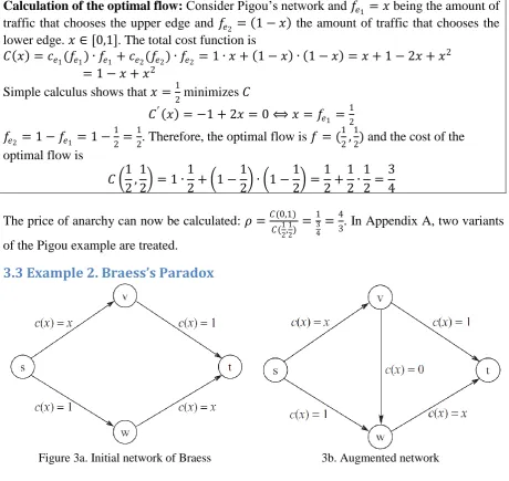
3.2 Example 1. Pigou’s example

[image:6.595.79.519.555.670.2]

Consider the network in Figure 2a. It was analyzed by Pigou (1920), the first person to study nonatomic selfish routing (Roughgarden, 2007).

Figure 2a. Pigou’s example 2b. A nonlinear variant of Pigou’s example.

There is only one commodity, from 𝑠 to 𝑡, with two possible paths. The upper edge, 𝑒1, has

constant cost of 1. The lower edge, 𝑒2, has increasing costs as more players take this route.

(7)

5

If the traffic over the lower edge is less than 1, then that edge will be more favorable than the upper edge for any player. This strategy is the dominant strategy. But as every player chooses this strategy, the price of the lower path is just as high as the price of the upper path. By Definition 1, this is an equilibrium flow (see the first row in Table 1).

The second row shows another feasible flow, i.e. all the players choose the upper edge. This is no equilibrium flow since 𝑐𝑒1 1 = 1 and 𝑐𝑒2 0 = 0 and so 𝑐𝑒1 ≤ 𝑐𝑒2 for 𝑓𝑒1 > 0 does not hold. In this situation, any player would benefit from changing path since its cost will go from 1 to 𝑥 with 𝑥 ∈ [0,1).

The third and last row shows the cost of the optimal flow, which is 3₄.

Calculation of the optimal flow: Consider Pigou’s network and 𝑓𝑒1 = 𝑥 being the amount of traffic that chooses the upper edge and 𝑓_𝑒₂ = 1 − 𝑥 the amount of traffic that chooses the lower edge. 𝑥 ∈ [0,1]. The total cost function is

𝐶 𝑥 = 𝑐𝑒1(𝑓𝑒1) ∙ 𝑓𝑒1 + 𝑐𝑒2(𝑓𝑒2) ∙ 𝑓𝑒2 = 1 ∙ 𝑥 + 1 − 𝑥 ∙ 1 − 𝑥 = 𝑥 + 1 − 2𝑥 + 𝑥2 = 1 − 𝑥 + 𝑥2

Simple calculus shows that 𝑥 =1₂ minimizes 𝐶

𝐶′_{𝑥 = −1 + 2𝑥 = 0 ⟺ 𝑥 = 𝑓} 𝑒1 =

1 2

𝑓_𝑒₂ = 1 − 𝑓_𝑒₁ = 1 −1₂ =1₂. Therefore, the optimal flow is 𝑓 = (1₂,1₂) and the cost of the optimal flow is

𝐶 1 2,

1

2 = 1 ∙ 1

2+ 1 − 1

2 ∙ 1 − 1 2 =

1 2+

1 2∙

1 2=

3 4

The price of anarchy can now be calculated: 𝜌 =𝐶(0,1)

𝐶(1₂,1₂) = 1

3 4

= 4₃. In Appendix A, two variants

of the Pigou example are treated.

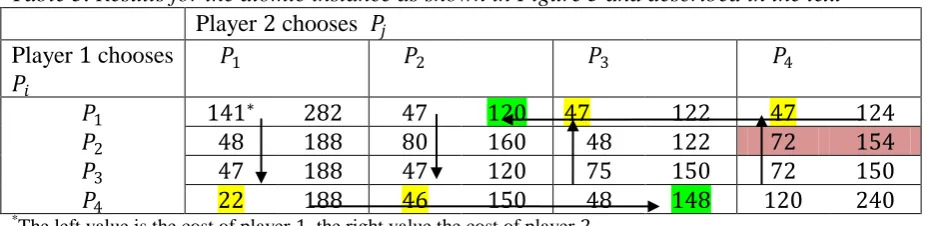
[image:7.595.68.529.347.782.2]

3.3 Example 2. Braess’s Paradox

Figure 3a. Initial network of Braess 3b. Augmented network

Table 1. Various feasible flows and the calculations of the total cost

Feasible flows

Calculations Total cost

𝑓_𝑒₁ 𝑓_𝑒₂ 𝑐_𝑃₁ 𝑓 = 𝑐_𝑒₁(𝑓_𝑒₁) 𝑐_𝑒₁(𝑓_𝑒₁) ∙ 𝑓_𝑒₁ 𝑐_𝑃₂ 𝑓 = 𝑐_𝑒₂(𝑓_𝑒₂) 𝑐_𝑒₂(𝑓_𝑒₂) ∙ 𝑓_𝑒₂

0 1 𝑐_𝑒₁ 0 = 1 1 ∙ 0 = 0 𝑐_𝑒₂ 1 = 1 1 ∙ 1 = 1 0 + 1 = 1 1 0 𝑐𝑒1 1 = 1 1 ∙ 1 = 1 𝑐𝑒2 0 = 0 0 ∙ 0 = 0 1 + 0 = 1

1 2

1

2 𝑐𝑒1

1

2 = 1 1 ∙ 1 2 =

1

2 𝑐𝑒2

1 2 =

1 2

1 2∙

1 2=

1 4

1 2+

1 4=

(8)

6

Another example of a nonatomic instance is the network of Braess’s Paradox. Braess (1968) was the first to discover that adding a supposedly beneficial edge to a network need not necessarily decrease the cost of an equilibrium flow. The current example uses other cost functions than the original example (according to Roughgarden (2007), the current variant was noted by L. Schulman (1999) in a personal communication between Roughgarden and Schulman).

See Figure 3a for the network and the cost functions. There is only one commodity, 𝑠 − 𝑡, and two paths that players of this commodity can choose. Call the upper path 𝑃₁ and the lower path 𝑃₂. Assume there is one unit of traffic, i.e. 𝑟 = 1. The cost of 𝑃₁ and 𝑃₂, 𝑐_𝑃₁and 𝑐_𝑃₂ respectively, is both 1 + 𝑥. (Note that this manner of writing the cost of a path, i.e. just summing the cost functions of the edges, is not always possible: if for example in Figure 3b, we change the cost function of edge 𝑠 − 𝑤, 𝑐_𝑒_𝑠−𝑤 𝑥 = 𝑥, then 𝑐𝑃2 𝑥 ≠ 2𝑥, since 𝑓𝑒𝑠−𝑤 is not necessarily equal to 𝑓𝑒𝑤 −𝑡)

If all traffic chooses 𝑃₁ in Figure 3a, the total cost of the flow is

𝐶 𝑓 = 𝑐_𝑒₁ 𝑓_𝑒₁ + 𝑐_𝑒₂ 𝑓_𝑒₂ ∙ 𝑓_𝑃₁ + 𝑐_𝑒₃ 𝑓_𝑒₃ + 𝑐_𝑒₄ 𝑓_𝑒₄ ∙ 𝑓_𝑃₂ = 𝐶 1,0 = 1 + 1 ∙ 1 + (1 + 0) ∙ 0 = 2

Players might reconsider their choice since deviating to 𝑃2 would decrease their cost

(𝑐_𝑃2(1,0) = 1 < 2 = 𝑐_𝑃1(1,0)). Players keep deviating from 𝑃₁ to 𝑃₂ until 𝑐_𝑃₁ = 𝑐_𝑃₂ (and vice versa). It is obvious that the equilibrium flow splits the traffic in half. At that point, both

paths have equal costs 𝑐𝑃1

1 2,

1

2 = 𝑐𝑃2

1 2,

1 2 =

1 2+ 1 =

3

2 so no player will benefit from

changing its path. The total cost is 𝐶 1₂,1₂ =3₂∙₂1+3₂∙1₂= 3₂.

In this network, the optimal flow coincides with the equilibrium flow. Therefore, the price of anarchy is equal to 1. This means that even though the players will exhibit selfish behavior, the overall cost will be minimal.

Calculation of the optimal flow in the network of Figure 3a: 𝑓𝑃1 = 𝑥 is the amount of traffic choosing 𝑃1, 𝑓𝑃2 = 1 − 𝑥 chooses 𝑃2.

𝐶 𝑥 = 𝑥 + 1 ∙ 𝑥 + 1 + 1 − 𝑥 ∙ 1 − 𝑥 = 𝑥 + 𝑥2_{+ 2 − 3𝑥 + 𝑥}2 _{= 2 − 2𝑥 + 2𝑥}2

Calculating the minimum:

𝐶′_{𝑥 = −2 + 4𝑥 = 0 ⟺ 𝑓}

𝑃1 = 𝑥 =

1

2, and 𝑓𝑃2 = 1 − 𝑓𝑃1 = 1 −

1 2=

1 2

Optimal flow: 𝑓 = (1₂,1₂).

Consider now Figure 3b. This is the original network with one added edge, 𝑒5, with zero cost.

The previous equilibrium does not hold. The new path, 𝑠 − 𝑣 − 𝑤 − 𝑡, 𝑃₃, has lower cost than either 𝑃₁ or 𝑃₂. Defining the cost of the third path, 𝑃₃, as function of the amount of traffic taking the other two paths, we can calculate the equilibrium flow as follows:

Calculation of the equilibrium flow in the network of Figure 3b:

The flow over 𝑃₁ and 𝑃₂ will be equal since the edge cost functions are equal, call it 𝑓_𝑃₁ = 𝑓𝑃2 = 𝑥, 𝑓𝑃3 = 1 − 2𝑥.

𝑐_𝑃₁ 𝑥, 𝑥, 1 − 2𝑥 = 𝑐_𝑃₂ 𝑥, 𝑥, 1 − 2𝑥 = 𝑥 + 1 − 2𝑥 + 1 = 2 − 𝑥 𝑐_𝑃₃ 𝑥, 𝑥, 1 − 2𝑥 = 𝑥 + 1 − 2𝑥 + 0 + 𝑥 + 1 − 2𝑥 = 2 − 2𝑥 In an equilibrium flow, 𝑐_𝑃₁ = 𝑐_𝑃₃ (if 𝑓_𝑃₁, 𝑓_𝑃₂ > 0) so

2 − 𝑥 = 2 − 2𝑥 ⟺ −𝑥 = −2𝑥 ⟺ 𝑥 = 0

(9)

7

𝐶 0,0,1 = 𝑐_𝑃1 0,0,1 ∙ 0 + 𝑐_𝑃2 0,0,1 ∙ 0 + 𝑐_𝑃3(0,0,1) ∙ 1 = 1 + 1 ∙ 0 + 1 + 1 ∙ 0 + 1 + 0 + 1 ∙ 1 = 2

The optimal flow can be calculated as follows:

Calculation of the optimal flow in the network of Figure 3b: The cost function (using equation (2)) is as follows:

𝐶 𝑓 = 𝑥₁+ 𝑥₃ 𝑥₁+ 𝑥₃ + 1 ∙ 𝑥₁+ 1 ∙ 𝑥₂+ 𝑥₂+ 𝑥₃ (𝑥₂+ 𝑥₃)

where 𝑥₁ is 𝑓_𝑃₁, 𝑥₂ = 𝑓_𝑃₂, 𝑥₃ = 𝑓_𝑃₃, the first term is the cost of edge 𝑠 − 𝑣, the second term of edge 𝑣 − 𝑡, the third of 𝑠 − 𝑤 and the fourth of 𝑤 − 𝑡. The edge 𝑣 − 𝑤 has zero cost, therefore it is not added.

𝐶 𝑓 = 𝑥1+ 𝑥2+ 𝑥12 + 𝑥22 + 2𝑥32+ 2𝑥1𝑥3+ 2𝑥2𝑥3

∇2_{𝐶 𝑓 =}2 0 2_{0 2 2}

2 2 4

which has eigenvalues 𝜆₁ = 0, 𝜆₂ = 4, 𝜆₃ = 4, making ∇2_{𝐶 𝑓 a positive semidefinite matrix}

for any (feasible) 𝑓. This implies that 𝐶(𝑓) is convex. Also, 𝑥₁+ 𝑥₂+ 𝑥₃ = 1 is a convex function. So

min_𝑓∈ℝ₊3 𝑥₁+ 𝑥₂+ 𝑥₁2+ 𝑥₂2+ 2𝑥₃2+ 2𝑥₁𝑥₃ + 2𝑥₂𝑥₃ s.t. 𝑥₁+ 𝑥₂+ 𝑥₃ = 1 is a convex program. Rewrite the equality constraint:

𝑔₁ 𝑓 = 𝑥1+ 𝑥2+ 𝑥3− 1 ≤ 0

𝑔₂ 𝑓 = 1 − 𝑥1− 𝑥2− 𝑥3 ≤ 0

The KKT-condition reads:

1 + 2𝑥1+ 2𝑥3

1 + 2𝑥2+ 2𝑥3

4𝑥₃+ 2𝑥₁+ 2𝑥₂ = −𝑦1 1 1 1

− 𝑦2

−1 −1 −1

The top two equations read:

1 + 2𝑥1 + 2𝑥3 = −𝑦1+ 𝑦2

1 + 2𝑥₂+ 2𝑥₃ = −𝑦₁+ 𝑦₂ ⟹ 𝑥1 = 𝑥2

The third equation can be rewritten as

4𝑥3+ 4𝑥1 = −𝑦1+ 𝑦2 ⟹ 4𝑥3 + 4𝑥1 = 1 + 2𝑥1+ 2𝑥3 ⟺ 2𝑥3+ 2𝑥1 = 1

The equality-constraint can be written as 1 = 𝑥3+ 2𝑥1. Together:

1 = 2𝑥3+ 2𝑥1

1 = 𝑥₃+ 2𝑥₁ if 𝑥1 = 0, then the system is insolvable, so 𝑥1 > 0

It is only solvable if 𝑥₃ = 0 and 1 = 2𝑥₁ ⟺ 𝑥₁ = 𝑥₂ =1₂. Solution to the minimization problem: 𝑓∗ _{= (}1

2, 1 2, 0).

𝐶 1 2,

1

2, 0 = 1 2+ 1 ∙

1

2+ 1 + 1 2 ∙

1 2+

1 2+ 0 +

1 2 ∙ 0 =

3 2∙

1 2+

3 2∙

1

2+ 1 ∙ 0 = 3 2

The price of anarchy is 𝜌 =_𝐶(𝑓𝐶(𝑓)_∗₎= 𝐶(0,01)

𝐶(1₂,1₂,0)= 2

3 2

= 4₃.

3.4 Existence and uniqueness of equilibrium flows

Any nonatomic instance admits an equilibrium. Furthermore, any equilibrium flow in a nonatomic instance is essentially unique, which means that there might be several equilibria in an instance but they all have the same total cost. This part is going to prove these claims.

Recall Definition 2. Flow 𝑓∗_{is optimal if it is feasible and minimizes}

(10)

8

𝑐𝑒 𝑓𝑒 𝑓𝑒 is the contribution to the total cost of the flow of edge 𝑒. Call the derivative of this

contribution ‘the marginal cost function’, i.e. 𝑐_𝑒∗_𝑓

𝑒 = 𝑐𝑒 𝑓𝑒 𝑓𝑒 ′ = 𝑐𝑒 𝑓𝑒 + 𝑓𝑒 ∙ 𝑐𝑒′(𝑓𝑒)

This marginal cost function indicates how much the contribution to the total cost increases as more traffic uses the edge. 𝑐𝑒∗ is always positive as 𝑐𝑒 𝑓𝑒 𝑓𝑒 is always increasing.

Let 𝑐_𝑃∗ 𝑓 = _𝑒∈𝑃𝑐_𝑒∗(𝑓_𝑒) define the sum of the marginal costs of the edges in the path 𝑃 with respect to the flow 𝑓. If we are dealing with an optimal flow, the sum over all 𝑐𝑃(𝑓) ∙ 𝑓𝑃

is minimized. This means that the marginal cost function over two (or more) paths that are in use must be equal. If they are not, then a player can switch to the path where the marginal cost function is lower and thereby decreasing the total cost (i.e. if one unit of traffic will induce 5 extra units to the total cost on 𝑃₁ and 4 extra units on 𝑃₂, changing from 𝑃₁ tot 𝑃₂ will decrease the total cost by 1). An unused path must always have an equal or a higher marginal cost for the same reasons. More formally:

Proposition 1 (Characterization of optimal flows) [R18.9] Let (𝐺, 𝑟, 𝑐) be a nonatomic instance such that, for every edge 𝑒, the function 𝑐_𝑒 𝑓_𝑒 𝑓_𝑒 is convex and continuously differentiable. Let 𝑐𝑒∗ denote the marginal cost function of the edge 𝑒. Then 𝑓∗ is an optimal

flow for (𝐺, 𝑟, 𝑐, ) if and only if, for every commodity 𝑖 ∈ {1, … , 𝑘} and every pair 𝑃, 𝑃 ∈ 𝒫𝑖

of 𝑠𝑖− 𝑡𝑖 paths with 𝑓𝑃∗ > 0,

𝑐_𝑃∗_𝑓∗_{≤ 𝑐} 𝑃 ∗(𝑓∗)

Proof: It has already been proven before that the feasible set of flows is convex. It is assumed that 𝑐_𝑒 𝑓_𝑒 𝑓_𝑒 is convex, and the sum of convex functions is in turn convex (i.e. 𝐶 𝑓 = 𝑒∈𝐸𝑐_𝑒 𝑓𝑒 𝑓𝑒 is convex). Consider the following convex program

min

𝑓 𝐶 𝑓 = 𝑐𝑒 𝑓𝑒 𝑓𝑒 𝑒∈𝐸

𝑓𝑃

𝑃∈𝒫𝑖 = 𝑟𝑖 for all 1 ≤ 𝑖 ≤ 𝑘 𝑓_𝑃 ≥ 0 for all 𝑃 ∈ 𝒫

𝑓 ∈ ℝ 𝒫

Flow 𝑓 is optimal if and only if it satisfies the KKT-conditions. Denote the objective function and constraints of the program as follows:

𝐶 𝑓 = 𝑐𝑒 𝑓𝑒 𝑓𝑒 𝑒∈𝐸

𝑔_𝑃 𝑓 = −𝑓_𝑃 ≤ 0 for all 𝑃 ∈ 𝒫

𝑕𝑖 𝑓 = 𝑃∈𝒫𝑖𝑓𝑃 − 𝑟𝑖 = 0, for all 1 ≤ 𝑖 ≤ 𝑘

So 𝑓 is optimal if and only if there exist multipliers 𝜇_𝑃, 𝜆_𝑖 such that

∇𝐶 𝑓 = − 𝜆_𝑃

𝑃∈𝒫

∇𝑔_𝑃 𝑓 − 𝜇_𝑖

𝑘

𝑖=1

∇𝑕_𝑖(𝑓)

𝜆_𝑃 ≥ 0, 𝜆_𝑃𝑔_𝑃 𝑓 = 0

Suppose that 𝑓 is optimal, then there exist 𝜆_𝑃, 𝜇_𝑖 that satisfy the KKT-conditions. Considering the conditions per path:

∇𝐶 𝑓 _𝑃 = 𝑐_𝑒 𝑓_𝑒 𝑓_𝑒 ′

𝑒∈𝑃

= 𝑐_𝑒∗_(𝑓 𝑒) 𝑒∈𝑃

= 𝑐_𝑃∗_(𝑓)

∇𝑔_𝑃 𝑓 _𝑃 = −1

∇𝑕_𝑖 𝑓 _𝑃 = 1 if 𝑃 ∈ 𝒫_{0 if 𝑃 ∉ 𝒫}𝑖

𝑖

(11)

9 𝑓𝑃

𝑃∈𝒫_𝑖 = 𝑓𝑃1+ 𝑓𝑃2+ 𝑓𝑃3. So differentiating with respect to the flow of some path in 𝒫 yields 1 if the path is in 𝒫_𝑖 and 0 if it is not)

For any path 𝑃 ∈ 𝒫_𝑖, we have

𝑐_𝑃∗_{𝑓 = 𝜆} 𝑃− 𝜇𝑖

𝜆𝑃 ≥ 0, −𝜆𝑃𝑓𝑃 = 0

Consider two paths in 𝒫_𝑖, 𝑃, 𝑃 ∈ 𝒫_𝑖 where at least 𝑃 routes some traffic: 𝑓_𝑃 > 0. Then – 𝜆_𝑃𝑓_𝑃 = 0 can only hold if 𝜆_𝑃 = 0, so

𝑐_𝑃∗_{𝑓 = −𝜇} 𝑖

𝑐_𝑃∗ 𝑓 = 𝜆𝑃 − 𝜇𝑖

Since 𝜆_𝑃 ≥ 0 , it follows that 𝑐_𝑃∗ _{≤ 𝑐} 𝑃 ∗.

To proof the reverse, assume that for 𝑃, 𝑃 ∈ 𝒫_𝑖, 𝑓_𝑃 > 0, the following holds: 𝑐_𝑃∗ ≤ 𝑐_𝑃∗ and thus: 𝑐_𝑃∗ − 𝑐_𝑃∗ _{≥ 0. We need to find multipliers 𝜆}

𝑃 and 𝜇𝑖 such that the KKT-condition holds.

Since 𝑓 is feasible, every commodity has at least one path such that 𝑓𝑃1 > 0. Therefore, set 𝜆_𝑃 = 𝑐_𝑃∗_{𝑓 − 𝑐}

𝑃1

∗ _(𝑓)

𝜇𝑖 = −𝑐𝑃∗1(𝑓)

I will check that the KKT-conditions are satisfied: Take 𝑃, 𝑃 ∈ 𝒫𝑖, and some 𝑃1 ∈ 𝒫𝑖 such

that 𝑓_𝑃₁ > 0. We know 𝑐_𝑃∗₁(𝑓) ≤ 𝑐_𝑃∗(𝑓) for any 𝑃 ∈ 𝒫_𝑖. Therefore 𝜆_𝑃 ≥ 0. If 𝑓_𝑃 > 0, then 𝑐_𝑃∗₁_{𝑓 = 𝑐}

𝑃∗ 𝑓 ⟹ 𝜆𝑃 = 0 ⟹ −𝜆𝑃𝑓𝑃 = 0. If 𝑓𝑃 = 0, then also −𝜆𝑃𝑓𝑃 = 0, so the

conditions −𝜆_𝑃𝑓_𝑃 = 0 and 𝜆_𝑃 ≥ 0 are satisfied. Also, for any 𝑃 ∈ 𝒫_𝑖,

∇𝐶 𝑓 _𝑃 = −𝜆_𝑃∙ ∇𝑔_𝑃 𝑓 _𝑃− 𝜇_𝑖∙ ∇𝑕_𝑖 𝑓 _𝑃 ⟹ 𝑐_𝑃∗_{𝑓 = −𝜆}

𝑃 ∙ −1 − 𝜇𝑖∙ 1 = 𝜆𝑃− 𝜇𝑖 = 𝑐𝑃∗ 𝑓 − 𝑐𝑃∗1 𝑓 + 𝑐𝑃∗1 𝑓 = 𝑐𝑃∗(𝑓) As the KKT-conditions are satisfied, it follows that 𝑓 is optimal. ∎

(Proof adapted from Olsthoorn, 2012, first proof given by Beckman, 1956)

Proposition 1 looks a lot like the definition of an equilibrium flow: the optimal flow of (𝐺, 𝑟, 𝑐) is the equilibrium flow for (𝐺, 𝑟, 𝑐∗_{). This idea is formalized in Corollary 1:}

Corollary 1 (Equivalence of equilibrium and optimal flows) [R18.10] Let (𝐺, 𝑟, 𝑐) be a nonatomic instance such that, for every edge 𝑒, the function 𝑐𝑒 𝑓𝑒 𝑓𝑒 is convex and

continuously differentiable. Let 𝑐_𝑒∗_{denote the marginal cost function of the edge}_{𝑒. Then}_𝑓∗

is an optimal flow for (𝐺, 𝑟, 𝑐) if and only if it is an equilibrium flow for (𝐺, 𝑟, 𝑐∗_).

(First proof given by Beckman, 1956)

To proof the existence of equilibrium flows in nonatomic instances, one can use Corollary 1. We are looking for some function 𝑕_𝑒 for every edge such that its derivative is 𝑐_𝑒. The only assumption on 𝑕_𝑒 would be that 𝑕_𝑒 𝑓_𝑒 is convex. An obvious candidate is 𝑕_𝑒 𝑓_𝑒 = ∫ 𝑐₀𝑓𝑒 𝑒 𝑥 𝑑𝑥. Since 𝑐𝑒 is continuous and nondecreasing for every edge 𝑒, every function 𝑕𝑒 is

both continuously differentiable and convex (𝑕_𝑒′ _{= 𝑐}

𝑒 for every 𝑒 ∈ 𝐸).

Next we are going to define the potential function of a nonatomic instance. The idea of the potential function is that the global minima of this function are precisely the equilibrium

flows of the nonatomic instance. Define the potential function Φ 𝑓 = 𝑒∈𝐸∫ 𝑐₀𝑓𝑒 𝑒(𝑥)𝑑𝑥.

Since this is a sum of convex functions, the potential function is also convex. By using Proposition 1, one can see that if we replace 𝑓𝑒 ∙ 𝑐𝑒(𝑓𝑒) with 𝑕𝑒 𝑓𝑒 for every 𝑒 ∈ 𝐸, then

𝑕_𝑒′_(𝑓

𝑒) = 𝑐𝑒(𝑓𝑒). In Corollary 1, 𝑕𝑒 plays the role of 𝑐𝑒 𝑓𝑒 𝑓𝑒.

(12)

10

Proposition 2 (Potential function for equilibrium flows) [R18.11] Let (𝐺, 𝑟, 𝑐) be a nonatomic instance. A flow feasible for (𝐺, 𝑟, 𝑐) is an equilibrium flow if and only if it is a global minimum of the corresponding potential function Φ given by

Φ 𝑓 = 𝑐𝑒(𝑥)𝑑𝑥 𝑓𝑒

0 𝑒∈𝐸

(First proof given by Beckman, 1956)

In appendix B one can find the calculations of the equilibrium flow using the potential function for the two examples of sections 3.2 and 3.3.

Now we have all tools to prove the following theorem:

Theorem 1 (Existence and uniqueness of equilibrium flows) [R18.8] Let (𝐺, 𝑟, 𝑐) be a nonatomic instance.

(a) The instance (𝐺, 𝑟, 𝑐) admits at least one equilibrium flow.

(b) If 𝑓 and 𝑓 are equilibrium flows for 𝐺, 𝑟, 𝑐 , then 𝑐_𝑒 𝑓_𝑒 = 𝑐_𝑒(𝑓 _𝑒) for every edge 𝑒.

Proof: The set of feasible flows is bounded (i.e. any 𝑓_𝑃 is bounded by 0 and 𝑟_𝑖) and closed (since any 𝑓_𝑃 ∈ [0, 𝑟_𝑖]) and therefore compact. It is a subset of ℝ₊ 𝒫 . Since edge cost functions are continuous, the 𝑕𝑒 functions are continuous and therefore the potential function

Φ is continuous as well. Weierstrass’s Theorem tells us that a continuous function on a compact set always admits at least one minimum on that set. So, the potential function on the compact set of feasible flows admits at least one minimum. By Proposition 2, this minimum is an equilibrium flow for the atomic instance (𝐺, 𝑟, 𝑐). Thus, part (a) is proven.

We know that the potential function is convex. This means that any minimum of the function is a global minimum and that any point on the line between any minima also is a global minimum. Suppose 𝑓 and 𝑓 are equilibrium flows for (𝐺, 𝑟, 𝑐), then they are global minima for Φ(𝑓). Then for any 𝜆 ∈ [0,1], 𝜆𝑓 + (1 − 𝜆)𝑓 is also a global minimum of Φ(𝑓).

Φ 𝜆𝑓 + 1 − 𝜆 𝑓 = 𝜆Φ 𝑓 + (1 − 𝜆)Φ(𝑓 )

since Φ is constant between 𝑓 and 𝑓 . The sum of |𝐸| convex summands can only be linear if every summand is linear too (If a function is strictly convex, then its derivative is not constant but increasing over the entire interval and the sum of two increasing functions is also increasing. Therefore the sum of two strictly convex functions can never be a constant function). It is linear between 𝑓𝑒 and 𝑓 𝑒. If an integral over 𝑐𝑒 is linear between 𝑓𝑒 and 𝑓 𝑒, then

𝑐_𝑒 is constant between 𝑓_𝑒 and 𝑓 _𝑒, meaning 𝑐_𝑒 𝑓_𝑒 = 𝑐_𝑒(𝑓 _𝑒) for every edge 𝑒, proving part (b). ∎

(Proof adapted from Roughgarden, 2007, first proof given by Beckman,1956)

If 𝑐𝑒 𝑓𝑒 = 𝑐𝑒(𝑓 𝑒) for every edge 𝑒, then 𝑐𝑃 𝑓 = 𝑐𝑃(𝑓 ) for 𝑓, 𝑓 two equilibrium flows. If the

flows are distinct, then 𝑓_𝑒 ≠ 𝑓 _𝑒 for at least two edges. 𝑐_𝑒 𝑓_𝑒 = 𝑐_𝑒(𝑓 _𝑒) can only hold if 𝑐_𝑒 is constant between 𝑓_𝑒 and 𝑓 _𝑒. Therefore, there is only one unique equilibrium flow if the cost functions are strictly increasing. We can have two distinct equilibrium flows if there is at least one edge cost function that is not strictly increasing.

Furthermore, since 𝑐𝑒 𝑓𝑒 = 𝑐𝑒(𝑓 𝑒) holds for every edge 𝑒, also 𝑐𝑃 𝑓 = 𝑐𝑃(𝑓 ) holds for

(13)

11 𝐶 𝑓 = 𝑐𝑃 𝑓 𝑓𝑃

𝑃∈𝒫

= 𝐿𝑖 ∙ 𝑓𝑃 𝑃∈𝒫𝑖

𝑘

𝑖=1

= 𝐿𝑖∙ 𝑓𝑃 𝑃∈𝒫𝑖

𝑘

𝑖=1

= 𝐿𝑖 ∙ 𝑟𝑖 𝑘

𝑖=1

= 𝐿𝑖∙ 𝑓 𝑃 𝑃∈𝒫𝑖

𝑘

𝑖=1

= 𝐿𝑖 ∙ 𝑓 𝑃 𝑃∈𝒫𝑖

𝑘

𝑖=1

= 𝑐𝑃 𝑓 𝑓 𝑃 𝑃∈𝒫

= 𝐶(𝑓 )

Therefore, for any two or more (distinct) equilibrium flows, 𝐶 𝑓 = 𝐶(𝑓 ).

3.5 The price of anarchy

This section gives a short analysis of the price of anarchy in nonatomic instances. The price of anarchy (𝜌) is defined as the ratio of the objective value of an equilibrium flow and the objective value of the optimal flow (see Definition 2). The price of anarchy in the two examples above was 4₃. In this section I will show that in any nonatomic instance with only

affine cost functions, the price of anarchy is at most 4₃.

For any nonatomic instance, the potential function gives a rough upper bound on the price of anarchy.

Theorem 2 (Potential function upper bound) [R18.16] Let (𝐺, 𝑟, 𝑐) be a nonatomic instance, and suppose that 𝑥 ∙ 𝑐_𝑒 𝑥 ≤ 𝛾 ∙ ∫ 𝑐₀𝑥 𝑒(𝑦)𝑑𝑦 for all 𝑒 ∈ 𝐸 and 𝑥 ≥ 0. Then the price

of anarchy of (𝐺, 𝑟, 𝑐) is at most 𝛾.

Proof: Let 𝑓 be an equilibrium flow and 𝑓∗ an optimal flow for (𝐺, 𝑟, 𝑐). 𝐶 𝑓 ≤ 𝛾 ∙ Φ 𝑓 ≤ 𝛾 ∙ Φ 𝑓∗_{≤ 𝛾 ∙ 𝐶(𝑓}∗₎

The first inequality follows from the hypothesis (summing over all 𝑒 does not change the inequality sign), the second from the fact that 𝑓 is a global minimizer of Φ according to Proposition 2, and the third follows from the next observation: Since 𝑐_𝑒 is nonnegative and nondecreasing, 𝑐_𝑒(𝑓_𝑒)𝑓_𝑒 will always be at least as big as ∫ 𝑐₀𝑓𝑒 𝑒(𝑥)𝑑𝑥,

∫ 𝑐₀𝑓𝑒 𝑒(𝑥)𝑑𝑥≤ 𝑐𝑒 𝑓𝑒 𝑓𝑒 (equality holds when 𝑐𝑒 is constant between 0 and 𝑓𝑒)

𝐶 𝑓 ≤ 𝛾 ∙ 𝐶 𝑓∗_{⟺ 𝜌(𝐺, 𝑟, 𝑐) =} 𝐶 𝑓

𝐶 𝑓∗ ≤ 𝛾. ∎

(Proof adapted from Roughgarden, 2007, first proof by Roughgarden and Tardos, 2002)

Note that this upper bound 𝛾 equals 2 when all cost functions are linear.

An upper bound on 𝝆(𝑮, 𝒓, 𝒄) is 𝟐 for an affine nonatomic instance

We are looking for a 𝛾 as small as possible for which 𝑥 ∙ 𝑐𝑒 𝑥 ≤ 𝛾 ∙ ∫ 𝑐₀𝑥 𝑒(𝑦)𝑑𝑦 holds for

any 𝑐_𝑒 𝑥 = 𝑎_𝑒𝑥 + 𝑏_𝑒, and 𝑎_𝑒, 𝑏_𝑒 ≥ 0.

𝑥 ∙ 𝑐_𝑒 𝑥 ≤ 𝛾 ∙ 𝑐_𝑒(𝑦)𝑑𝑦

𝑥

0

⟹ 𝑎_𝑒𝑥2_{+ 𝑏}

𝑒𝑥 ≤ 𝛾(

1

2𝑎𝑒𝑥2+ 𝑏𝑒𝑥) This is true for any 𝑎_𝑒, 𝑏_𝑒 ≥ 0 for 𝛾 = 2 (an upper bound for 𝛾).

Set 𝑏𝑒 = 0, then a lower bound on 𝛾 is 𝛾 = 2. Together, 𝛾 = 2 is a tight bound for the price

of anarchy in an atomic instance with only linear cost functions.

In fact, for any polynomial cost function, 𝛾 = 𝑝 + 1 where 𝑝 is the degree of the polynomial.

(14)

12

nonatomic instance with polynomial cost functions with nonnegative coefficients and degree at most 𝑝, then the price of anarchy of (𝐺, 𝑟, 𝑐) is at most 𝑝 + 1.

Proof: According to Theorem 2, if we can find a 𝛾 such that 𝑥 ∙ 𝑐_𝑒 𝑥 ≤ 𝛾 ∙ ∫ 𝑐₀𝑥 _𝑒(𝑦)𝑑𝑦 for all 𝑒, then that 𝛾 is the upper bound on the price of anarchy.

𝑐_𝑒 𝑥 = 𝑎_𝑝𝑥𝑝 _{+ 𝑎}

𝑝−1𝑥𝑝−1+ ⋯ + 𝑎1𝑥 + 𝑎0

𝑥 ∙ 𝑐_𝑒 𝑥 = 𝑎_𝑝𝑥𝑝+1_{+ 𝑎}

𝑝−1𝑥𝑝 + ⋯ + 𝑎0𝑥

≤ 𝛾 𝑐_𝑒(𝑦)𝑑𝑦

𝑥

0

= 𝛾( 1

𝑝 + 1𝑎𝑝𝑥𝑝+1+ 1

𝑝𝑎𝑝−1𝑥𝑝 + ⋯ + 𝑎0𝑥) This inequality holds for any polynomial if 𝛾 = 𝑝 + 1:

𝑎_𝑝𝑥𝑝+1_{+ 𝑎}

𝑝−1𝑥𝑝 + ⋯ + 𝑎0𝑥 ≤ 𝑎𝑝𝑥𝑝+1+

𝑝 + 1

𝑝 𝑎𝑝−1𝑥𝑝 + ⋯ + (𝑝 + 1)𝑎0𝑥 is true since

𝑎𝑝𝑥𝑝+1 = 𝑎𝑝𝑥𝑝+1, 𝑎𝑝−1𝑥𝑝 ≤

𝑝 + 1

𝑝 𝑎𝑝−1𝑥𝑝, … , 𝑎0𝑥 ≤ 𝑝 + 1 𝑎0𝑥 Therefore, 𝛾 = 𝑝 + 1 is an upper bound on 𝛾.

Set all coefficients 𝑎𝑗, 𝑗 = 0, … , 𝑝 − 1 , equal to zero. Then

𝑎_𝑝𝑥𝑝+1_{≤ 𝛾} 1

𝑝 + 1𝑎𝑝𝑥𝑝+1

This is true if 𝛾 at least equals 𝑝 + 1, making 𝛾 = 𝑝 + 1 an lower bound on 𝛾. Together 𝛾 = 𝑝 + 1 is a tight bound for the price of anarchy of (𝐺, 𝑟, 𝑐). ∎

The potential function already gives a good upper bound estimate, but it is not optimal yet. In the next part, I will show that there is a tight bound on the price of anarchy that is even lower than 𝛾.

The idea is as follows: first we formalize a lower bound by using Pigou-like networks (i.e. a network with two vertices and two edges, one commodity with 𝑟 units of traffic and cost functions 𝑐₁ 𝑥 = 𝑐(𝑟), 𝑐2 𝑥 = 𝑐(𝑥)). Then we establish an upper bound on the price of

anarchy in general multicommodity flow networks. This bound was called the anarchy value by Roughgarden (2003) but later he renamed it to the Pigou bound (Roughgarden, 2007).

Definition 4 (Pigou bound) [R18.18] Let 𝒞 be a nonempty set of cost functions. The Pigou bound 𝛼(𝒞) for 𝒞 is

𝛼 𝒞 = sup

𝑐∈𝒞 𝑥,𝑟≥0sup

𝑟 ∙ 𝑐 𝑟

𝑥 ∙ 𝑐 𝑥 + 𝑟 − 𝑥 𝑐 𝑟 , with the understanding that 0₀ = 1.

The fraction is the price of anarchy: the numerator is the cost of the equilibrium flow in a Pigou-like network, where all the traffic is routed over the lower edge. The denominator is the cost of the optimal flow: 𝑥 units are routed over the lower edge and 𝑟 − 𝑥 units are routed over the upper edge. The next proposition shows that this Pigou bound is a lower bound on the price of anarchy.

(15)

13

Proof: Fix a choice of 𝑐 ∈ 𝒞 and 𝑥, 𝑟 ≥ 0. Since 𝑐 is nondecreasing, sup𝑐∈𝒞sup𝑥,𝑟≥0_{𝑥∙𝑐 𝑥 + 𝑟−𝑥 𝑐 𝑟}𝑟∙𝑐 𝑟 = 1 if 𝑥 ≥ 𝑟

If 𝑥 = 𝑟, _{𝑥∙𝑐 𝑥 + 𝑟−𝑥 𝑐 𝑟}𝑟∙𝑐 𝑟 = 𝑟∙𝑐 𝑟 _{𝑟∙𝑐 𝑟}= 1

and if 𝑥 > 𝑟, _{𝑥∙𝑐 𝑥 + 𝑟−𝑥 𝑐 𝑟}𝑟∙𝑐 𝑟 = _{𝑥∙ 𝑐 𝑥 −𝑐 𝑟 +𝑟∙𝑐 𝑟}𝑟∙𝑐 𝑟 and 𝑥 ∙ 𝑐 𝑥 − 𝑐 𝑟 ≥ 0 so the expression is at most 1. Therefore, we can assume that 𝑥 ≤ 𝑟.

Let 𝐺 be a Pigou-like network. The lower edge has cost function 𝑐2 𝑥 = 𝑐(𝑥) and the

upper edge has cost function 𝑐₁ 𝑥 = 𝑐(𝑟), 𝑐 ∈ 𝒞. Set the traffic rate to 𝑟. The equilibrium flow routes all the traffic over the lower edge, yielding cost 𝑟 ∙ 𝑐(𝑟). Any feasible flow routes 𝑥 units of traffic on the lower edge and 𝑟 − 𝑥 units on the upper edge. This yields cost 𝑥 ∙ 𝑐 𝑥 + 𝑟 − 𝑥 𝑐 𝑟 . By varying 𝑥, one can find the 𝑥 for which 𝑥 ∙ 𝑐 𝑥 + 𝑟 − 𝑥 𝑐 𝑟 is approximately minimal. Doing this for any 𝑐 ∈ 𝒞, one ends up with the price of anarchy being at least 𝛼(𝒞), or 𝜌 ≥ sup_𝑐∈𝒞sup_{𝑥,𝑟≥0}_{𝑥∙𝑐 𝑥 + 𝑟−𝑥 𝑐 𝑟}𝑟∙𝑐 𝑟 = 𝛼(𝒞). ∎

(Proof adapted from Roughgarden, 2007)

In order to proof that the Pigou bound is also an upper bound on the price of anarchy, we need an alternative characterization of the equilibrium flow.

Proposition 4 (Variational inequality characterization) [R18.20] Let 𝑓 be a feasible flow for the nonatomic instance (𝐺, 𝑟, 𝑐). If flow 𝑓 is an equilibrium flow, then

𝑐_𝑒 𝑓𝑒 𝑓𝑒 𝑒∈𝐸

≤ 𝑐_𝑒 𝑓𝑒 𝑓𝑒∗ 𝑒∈𝐸

holds for every flow 𝑓∗_{feasible for (𝐺, 𝑟, 𝑐).}

Proof: 𝑓 is an equilibrium flow if and only if 𝑐_𝑃 𝑓 ≤ 𝑐_𝑃(𝑓) for any 𝑃, 𝑃 ∈ 𝒫_𝑖, for any 𝑖, and for 𝑓_𝑃 > 0. 𝑐_𝑃 𝑓 = 𝑐_𝑃(𝑓) if in addition 𝑓_𝑃 > 0. If any traffic deviates, creating flow 𝑓∗, then that part costs an equal or higher amount since the price of the newly chosen path is equal or higher. Therefore,

𝑐𝑃 𝑓 𝑓𝑃 𝑃∈𝒫𝑖

≤ 𝑐𝑃 𝑓 𝑓𝑃∗ 𝑃∈𝒫𝑖

, ∀𝑖

Summing over 𝑖, it follows

𝑐𝑃 𝑓 𝑓𝑃 𝑃∈𝒫

≤ 𝑐𝑃 𝑓 𝑓𝑃∗ 𝑃∈𝒫

𝑐_𝑃 𝑓 𝑓_𝑃

𝑃∈𝒫

≤ 𝑐_𝑃 𝑓 𝑓_𝑃∗ 𝑃∈𝒫

⟺ 𝑐_𝑒 𝑓_𝑒

𝑒∈𝑃 𝑃∈𝒫

𝑓_𝑃 ≤ 𝑐_𝑒 𝑓_𝑒

𝑒∈𝑃

𝑓 _𝑃

𝑃∈𝒫

By reversing the order of summation, we obtain 𝑐_𝑒 𝑓𝑒 𝑓𝑒 𝑒∈𝐸

≤ 𝑐_𝑒 𝑓𝑒 𝑓𝑒∗ 𝑒∈𝐸

∎

(Proof adapted from Roughgarden, 2007, first proof by Smith,1979)

We can now show that the Pigou bound is also an upper bound on the price of anarchy.

(16)

14

Proof: Let 𝑓∗ and 𝑓 be optimal and equilibrium flows, respectively. Then

𝐶 𝑓∗_{= 𝑓} 𝑒∗𝑐𝑒 𝑓𝑒∗ 𝑒∈𝐸

= 𝑓𝑒∗𝑐𝑒 𝑓𝑒∗ + 𝑓𝑒 − 𝑓𝑒∗ 𝑐𝑒 𝑓𝑒

𝑐_𝑒 𝑓_𝑒 𝑓_𝑒 ∙ 𝑐𝑒 𝑓𝑒 𝑓𝑒 + 𝑓𝑒∗− 𝑓𝑒 𝑐𝑒 𝑓𝑒 𝑒∈𝐸

The fraction resembles the calculation of the total cost for a Pigou-like network with 𝑥 = 𝑓_𝑒∗

and 𝑟 = 𝑓_𝑒 (the fraction is raised to the power −1). The Pigou bound is the supremum of the fraction over all cost functions in 𝒞 and all 𝑥, 𝑟 ≥ 0, therefore

𝑓𝑒∗𝑐𝑒 𝑓𝑒∗ + 𝑓𝑒 − 𝑓𝑒∗ 𝑐𝑒 𝑓𝑒

𝑐_𝑒 𝑓𝑒 𝑓𝑒 ≥

1 𝛼(𝒞) for each edge 𝑒.

𝐶 𝑓∗_≥ 1

𝛼(𝒞) 𝑐𝑒 𝑓𝑒 𝑓𝑒

𝑒∈𝐸

+ 𝑓_𝑒∗_{− 𝑓}

𝑒 𝑐𝑒(𝑓𝑒) 𝑒∈𝐸

≥ 1

𝛼(𝒞) 𝑐𝑒 𝑓𝑒 𝑓𝑒

𝑒∈𝐸

= 𝐶(𝑓) 𝛼(𝒞) The last inequality follows from Proposition 4 that basically says: 𝑓_𝑒∗_{− 𝑓}

𝑒 𝑐𝑒(𝑓𝑒)

𝑒∈𝐸 ≥ 0.

𝐶 𝑓∗_≥ 𝐶(𝑓)

𝛼(𝒞)⟹ 𝜌 = 𝐶(𝑓)

𝐶(𝑓∗₎ ≤ 𝛼 𝒞

Therefore, 𝛼(𝒞) is an upper bound on the price of anarchy of (𝐺, 𝑟, 𝑐) with 𝑐 ∈ 𝒞. ∎ (Proof adapted from Roughgarden, 2007, first proof by Roughgarden, 2003)

Theorem 3 implies that the price of anarchy on any nonatomic instance is maximized by Pigou-like networks, no matter what network 𝐺 is considered (Roughgarden, 2003). The only restrictions are on the cost functions, and not on the network size, the network structure, nor the number of commodities. It is also remarkable that ‘the worst possible ratio’ for a certain instance with cost functions in 𝒞 can always be achieved with a network with only two parallel links (Roughgarden, 2003).

As a last example, we will show that the price of anarchy is at most 4₃ for nonatomic instances with affine cost functions.

Theorem 4 (The price of anarchy in affine nonatomic instances) If (𝐺, 𝑟, 𝑐) is a nonatomic instance with affine cost functions, then the price of anarchy of (𝐺, 𝑟, 𝑐) is at most

4 3.

Proof: Theorem 3 says that the price of anarchy of a nonatomic instance is at most 𝛼(𝒞). So for linear cost functions, we need to find 𝛼(𝒞) with 𝒞 the set of all possible affine cost functions.

𝛼 𝒞 = sup

𝑐∈𝒞 𝑥,𝑟≥0sup

𝑟 ∙ 𝑐 𝑟

𝑥 ∙ 𝑐 𝑥 + 𝑟 − 𝑥 𝑐 𝑟

with 𝑐 𝑟 = 𝑎𝑟 + 𝑏, 𝑐 𝑥 = 𝑎𝑥 + 𝑏, with 𝑎, 𝑏 ≥ 0 for any edge cost function. To maximize 𝑟∙𝑐 𝑟

𝑥∙𝑐 𝑥 + 𝑟−𝑥 𝑐 𝑟 over 𝑥, we need to minimize the following expression

𝑥 ∙ 𝑐 𝑥 + 𝑟 − 𝑥 𝑐 𝑟 = 𝑎𝑥2 _{+ 𝑏𝑥 + 𝑎𝑟}2_{+ 𝑏𝑟 − 𝑎𝑟𝑥 − 𝑏𝑥 = 𝑎𝑥}2 _{+ 𝑎𝑟}2_{+ 𝑏𝑟 − 𝑎𝑟𝑥}

Differentiating with respect to 𝑥 and equate to 0 yield 2𝑎𝑥 − 𝑎𝑟 = 0 ⟺ 𝑥 =1

2𝑟 𝛼 𝒞 = sup

𝑐∈𝒞

𝑟 ∙ 𝑐 𝑟 1

2 𝑟 ∙ 𝑐 12 𝑟 + 12 𝑟 𝑐 𝑟 = sup

𝑐∈𝒞

𝑎𝑟2_{+ 𝑏𝑟}

1

4 𝑎𝑟2+12 𝑏𝑟 +12 𝑎𝑟2+12 𝑏𝑟

= sup

𝑐∈𝒞

𝑎𝑟 + 𝑏 3

4 𝑎𝑟 + 𝑏

(17)

15 Then sup

𝑐∈𝒞 𝑎𝑟

3 4𝑎𝑟

= 13 4

= 4₃. ∎

(First proof given by Roughgarden and Tardos, 2002)

4. Atomic selfish routing

Most ingredients for atomic selfish routing are the same as for nonatomic selfish routing: There is a network 𝐺 = (𝑉, 𝐸) with a finite number of commodities 𝑖 = {1, … , 𝑘}, a positive amount of traffic per commodity 𝑟_𝑖 and each edge has a nondecreasing, continuous, nonnegative cost function 𝑐_𝑒: ℝ₊→ ℝ₊. We also denote an atomic instance by (𝐺, 𝑟, 𝑐). The main difference are the players: in an atomic instance, there are finitely many players, each assigned to one commodity, and each player directs its amount of traffic over just one path. This is the reason why sometimes this model is also called selfish unsplittable routing (e.g. see Fotakis, Kontogiannis, and Spirakis, 2005). There are 𝑘 players, each assigned to one of the 𝑘 commodities.

Flow is again denoted by 𝑓. Since the traffic is unsplittable and multiple players might be assigned the same source-sink pair, the flow per path has an extra index: 𝑓_𝑃(𝑖) indicates the

amount of traffic that player 𝑖 directs over path 𝑃, so 𝑓𝑃 = 𝑘𝑖=1𝑓𝑃 𝑖 . This vector is again

nonnegative. A flow is feasible if for each player 𝑖, 𝑓_𝑃 𝑖 equals 𝑟_𝑖 for one path 𝑃 ∈ 𝒫_𝑖 and 0 for 𝑃 ∈ 𝒫𝑖\𝑃.

The cost per path is the same as in a nonatomic instance: 𝑐𝑃 𝑓 = 𝑒∈𝑃𝑐𝑒(𝑓𝑒) where

𝑓_𝑒 = _{𝑃∈𝒫|𝑒∈𝑃}𝑓_𝑃. Also the total cost, the outcome of the game, is the same: 𝐶 𝑓 = 𝑐_𝑃 𝑓 𝑓𝑃

𝑃∈𝒫 or equivalently 𝐶 𝑓 = 𝑒∈𝐸𝑐𝑒 𝑓𝑒 𝑓𝑒.

Suppose there is a certain flow in a network. This flow is an equilibrium flow if no player can decrease its cost by deviating from its chosen path. Formally:

Definition 5 (Atomic equilibrium flow) [R18.5] Let 𝑓 be a feasible flow for the atomic instance (𝐺, 𝑟, 𝑐). The flow 𝑓 is an equilibrium flow if, for every player, 𝑖 ∈ {1, … , 𝑘} and every pair 𝑃, 𝑃 ∈ 𝒫_𝑖 of 𝑠_𝑖 − 𝑡_𝑖 paths with 𝑓_𝑃 𝑖 > 0,

𝑐𝑃 𝑓 ≤ 𝑐𝑃 𝑓

where 𝑓 is the flow identical to 𝑓 except that 𝑓 _𝑃 𝑖 = 0 and 𝑓 _𝑃 𝑖 = 𝑟𝑖.

The last line tells us that if only one player deviates from 𝑃 to 𝑃 , the flow changes from 𝑓 to 𝑓 and the only change is that all the traffic 𝑟𝑖 is now directed over 𝑃 instead of 𝑃. The definition

also tells us that in a equilibrium flow, a player has always chosen a path that has either equal or lower cost than when he would direct the traffic over another path.

In a nonatomic instance equilibria always existed and had equal costs; in an atomic instance, however, equilibria might not exist and if there exist multiple ones, the costs might be different. Both cases are explored in the following two examples.

4.1 Example 3. AAE example

(18)

[image:18.595.216.378.77.233.2]

16

Table 2. Results for the AAE example

Player 𝑖 1 or

2*

Cost per edge, 𝑐_𝑒 Cost per player 𝑖 (𝑐_𝑃, whichever 𝑃 𝑖

might choose)

Total cost 𝑐_𝑢𝑣 𝑥

= 𝑥 𝑐= 0 𝑣𝑢(𝑥) 𝑐= 𝑥 𝑢𝑤 𝑥 = 0 𝑐𝑤𝑢 𝑥 𝑐= 𝑥 𝑣𝑤 𝑥 𝑐= 𝑥 𝑤𝑣 𝑥 1 2 3 4

1111 1 1 1 1 1 1 1 1 4

1211 2 2 1 2 4 2 1 9

1121 1 0 2 1 1 2 2 1 6

1112 2 1 0 1 2 1 1 2 6

1221 2 0 1 1 1 2 3 1 1 7

1122 2 0 2 0 2 2 2 2 8

1212 3 0 2 3 5 2 3 13

1222 3 0 1 0 1 3 4 1 3 11

2111 2 1 2 4 2 1 2 9

2211 1 1 2 2 3 3 2 2 10

2121 0 3 2 5 3 3 2 13

2112 1 2 0 1 1 3 2 1 1 7

2221 1 0 2 1 2 4 2 2 2 10

2122 1 0 3 0 1 4 3 3 1 11

2212 2 1 0 2 1 2 4 2 2 10

2222 2 0 2 0 1 1 3 3 2 2 10

*₁_{means player}_𝑖_{takes the one-step path,}₂_{means he takes the two-step path. So for example,}₁₂₂₁_{means that}

player 1 and 4 take the one-step path and player 2 and 3 the two step path.

Example of calculations of one row in Table 2

Take a look at the row where player 1 and 3 take the one-step path and player 2 and 4 take the two-step path: 1212 (colored row). Player 1, 2 and 3 take edge 𝑢 − 𝑣, 𝑒𝑢−𝑣, its cost is

𝑐𝑢𝑣 3 = 3. 𝑒𝑤−𝑢 (player 4) costs 𝑐𝑤𝑢 1 = 0, 𝑒𝑣−𝑤 is taken by player 2 and 3, and costs

𝑐𝑣𝑤 2 = 2. All other edges are not used and cost 0.

The costs per player are calculated as follows:

𝐶𝑖 𝑓 = 𝑐𝑃(𝑓) ∙ 𝑓𝑃, with 𝑐𝑃 𝑓 = 𝑒∈𝑃𝑐𝑒(𝑓𝑒)

Player 1: 𝐶1 𝑓 = 𝑐𝑢𝑣 3 ∙ 𝑓𝑢𝑣 = 3 ∙ 1 = 3.

Player 2: 𝐶2 𝑓 = 𝑐𝑢𝑣 3 + 𝑐𝑣𝑤 2 ∙ 𝑓𝑢𝑣𝑤 = (3 + 2) ∙ 1 = 5

Player 3: 𝐶₃ 𝑓 = 𝑐𝑣𝑤 2 ∙ 𝑓𝑣𝑤 = 2 ∙ 1 = 2

Player 4: 𝐶₄ 𝑓 = 𝑐𝑤𝑢 1 + 𝑐𝑢𝑣 3 ∙ 𝑓𝑤𝑢𝑣 = (0 + 3) ∙ 1 = 3.

[image:18.595.66.530.259.557.2]

(19)

17 The total cost of the network is 3 + 5 + 2 + 3 = 13.

Obviously, every player choosing the one-step path, (1111) is both an equilibrium flow and an optimal flow. It is an equilibrium flow since if any player would deviate to the two-step path (e.g. player 1 deviating (2111) or player 3 (1121)) the cost for that path increases (in the first example, the cost of player 1 increases from 1 to 4. In the second example: player 3 increases its cost from 1 to 2).

Also, (2222) is an equilibrium flow. To check this, look up (1222), (2122), (2212), and (2221) and verify that the costs of the player that deviates from the two-step path to the one-step path are either equal or higher (as it says in Definition 4). However, its total cost is higher than the total cost of the first mentioned equilibrium flow.

For all flows, except for 1111 or (2222), one can make a sort of diagram for flows that would be a better choice for a certain player. Check for instance (2112). If player 1 changes path, he will decrease his cost from 3 to 2. If next player 4 changes path, he will decrease his cost from 2 to 1, and we end up in the optimal/equilibrium flow (1111). Any flow will end up at (1111), none end up at (2222).

This example has shown that in an atomic instance, there might exist several equilibria with different total cost.

The price of anarchy is 𝜌 =_𝐶(𝑓𝐶(𝑓)_∗₎=10₄ =5₂. Note that the ‘worst outcome value’

equilibrium flow is chosen to calculate the price of stability (see the discussion at the end of Section 3.1).

Later on, I will prove that in an unweighted atomic instance with affine cost functions, the price of anarchy is at most 5

2.

4.2 Example 4. Existence of equilibrium flows

Figure 5. Example of an atomic instance with no equilibrium flow

This example is created by Goemans, Mirrokni, and Vetta (2005). Consider the network shown in Figure 5. There are two players, both with source 𝑠 and sink 𝑡. Their traffic amounts are 𝑟1 = 1 and 𝑟2 = 2. Denote the following: 𝑃1: 𝑠 − 𝑡, 𝑃2: 𝑠 − 𝑣 − 𝑡, 𝑃3: 𝑠 − 𝑤 − 𝑡, 𝑃4: 𝑠 −

𝑣 − 𝑤 − 𝑡. Some results are shown in Table 3.

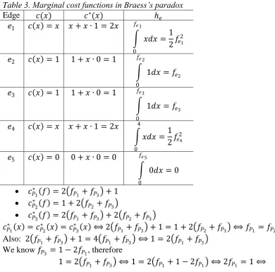
Example of calculations: Suppose player 1 takes path 2 and player 2 path 4 (colored cell in Table 3).

Cost player 1:

𝐶₁ 𝑓 = 𝑐_𝑠𝑣 𝑓_𝑠𝑣 + 𝑐_𝑣𝑡 𝑓_𝑣𝑡 ∙ 𝑓_𝑃₂ = 3 ∙ 32_{+ 1}2_{+ 44 ∙ 1 = 27 + 45 = 72}

Cost player 2:

[image:19.595.223.368.442.578.2]

(20)

[image:20.595.65.529.81.194.2]

18

Table 3. Results for the atomic instance as shown in Figure 5 and described in the text

Player 2 chooses 𝑃𝑗

Player 1 chooses 𝑃𝑖

𝑃1 𝑃2 𝑃3 𝑃4

𝑃1 141∗ 282 47 120 47 122 47 124

𝑃2 48 188 80 160 48 122 72 154

𝑃₃ 47 188 47 120 75 150 72 150

𝑃₄ 22 188 46 150 48 148 120 240

*

The left value is the cost of player 1, the right value the cost of player 2.

There is no equilibrium flow in this atomic instance:

 If player 2 chooses 𝑃₁ or 𝑃₂, the unique best response of player 1 is to choose 𝑃₄ (see yellow marking).

 If player 2 chooses 𝑃3 or 𝑃4, the unique best response of player 1 is to choose 𝑃1 (also

yellow marking).

 If player 1 chooses path 𝑃1, the unique best response of player 2 is to choose 𝑃2 (green

marking).

 If player 1 chooses path 𝑃₄, the unique best response of player 2 is to choose path 𝑃₃ (green marking).

Because of these four observations, there is no possible equilibrium flow: From any cell in the table, either player 1 or player 2 can decrease his cost by deviating from his chosen path. The possible deviations are indicated with arrows. The fact that the arrows are pointing in a circle at the middle top row and middle bottom row, and the fact that from any other cell the arrow points eventually to one of those four cells, imply that an equilibrium state is not possible.

There are two optimal flows: 𝑓∗ _{= (1,2,0,0) and 𝑓}∗ _{= (0,2,1,0). 𝐶 𝑓}∗_{= 𝐶 𝑓}∗_{= 167.}

4.3 Existence of equilibria

Why is there no equilibrium flow in Example 4 but does Example 3 admit two equilibria? The difference lies in the weights assigned to the players. You could call Example 3 an affine unweighted instance while Example 4 is a non-affine weighted instance. ‘Unweighted’ means that every player has the same amount of traffic to direct, i.e. 𝑟_𝑖 = 𝑅 for all 𝑖 = {1, … , 𝑘}. We will see that an atomic instance will admit an equilibrium flow if

1) All players have the same weight (𝑟_𝑖 is identical for all players) or

2) All cost functions are affine (𝑐_𝑒 𝑥 = 𝑎_𝑒𝑥 + 𝑏_𝑒, 𝑎_𝑒, 𝑏_𝑒 ≥ 0 for all edges).

4.3.1 Existence of equilibria: unweighted atomic instance

In this section, we prove Theorem 5 that says that any unweighted atomic instance admits at least one equilibrium flow. Formally:

Theorem 5 (Equilibrium flows in unweighted atomic instances) [R18.12] Let (𝐺, 𝑟, 𝑐) be an atomic instance in which every traffic amount 𝑟𝑖 is equal to a common positive value 𝑅.

Then (𝐺, 𝑟, 𝑐) admits at least one equilibrium flow.

Proof: Recall the potential function for a nonatomic instance. By discretizing it, one can proof Theorem 5. Assume for implicity that 𝑅 = 1. Set

Φ 𝑓 = 𝑐_𝑒(𝑖)

𝑓𝑒

𝑖=1 𝑒∈𝐸

(21)

19

Note how the integral part (of the continuous potential function) is substituted by a Riemann-sum with steps of 1. To prove the existence of an equilibrium flow, we prove that any global minimum of Φ 𝑓 is an equilibrium flow.

First, since there are a finite number of players and a finite number of paths to choose, the set of all feasible flows (ℱ) is finite. This means that the range of Φ is finite and thus a minimal value exists. Call the flow of minimal value 𝑓.

Now we prove that 𝑓 is an equilibrium flow in (𝐺, 𝑟, 𝑐). Assume to the contrary that 𝑓 is not an equilibrium flow. Then player 𝑖 could strictly decrease its cost by deviating from path 𝑃 to path 𝑃 (strictly: according to the definition, it is an equilibrium flow if all other paths have higher or equal cost. For a flow to be a nonequilibrium flow, at least one alternative path must have strictly lower cost). So we assume that there is a flow 𝑓 where one player chooses an alternative path 𝑃 with lower cost. This means:

𝑐𝑃 𝑓 > 𝑐𝑃 𝑓 ⟺ 0 > 𝑐𝑃 𝑓 − 𝑐𝑃 𝑓

The edges of 𝑃 are either in 𝑃 or they are not. 𝑃 and 𝑃 might have some edges in common, the cost of those edges does not change as player 𝑖 changes to path 𝑃 . This means that only the edges that they have not in common should be considered. First: When player 𝑖 deviates, he transfers his one unit from path 𝑃 to path 𝑃 . This means that edges that are now used extra have flow 𝑓_𝑒 + 1 (and edges that are not anymore used 𝑓_𝑒 − 1). Expressing the above-mentioned inequality in 𝑓 yields:

(4) 0 > 𝑐𝑃 𝑓 − 𝑐𝑃 𝑓 = 𝑐𝑒 𝑓𝑒 + 1 𝑒∈𝑃 \𝑃

− 𝑐𝑒 𝑓𝑒 𝑒∈𝑃\𝑃

The first sum is the cost all edges that are in 𝑃 but not in 𝑃, the second sum is the cost of all edges that are in 𝑃 but not in 𝑃 .

On the other hand, consider Φ. The new edges in 𝑃 (i.e. 𝑒 ∈ 𝑃 \𝑃) add to Φ(𝑓) one extra term, 𝑐𝑒(𝑓𝑒 + 1) (the +1 stems from 𝑅 = 1). The edges that are not anymore in 𝑃 , i.e.

𝑒 ∈ 𝑃\𝑃 , subtract a term of Φ(𝑓), namely 𝑐𝑒(𝑓𝑒) (since 𝑓𝑒 is now one less. The new sum for

this edge is 𝑓𝑖=1𝑒−1𝑐𝑒(𝑖)). The sum for common edges remains the same, i.e. 𝑓 𝑒 = 𝑓𝑒 ⟹

𝑐𝑒(𝑖) 𝑓 𝑒

𝑖=1 = 𝑓𝑖=1𝑒 𝑐𝑒(𝑖). Thus:

(5) Φ 𝑓 − Φ 𝑓 = 𝑐_𝑒 𝑓𝑒 + 1

𝑒∈𝑃 \𝑃

− 𝑐_𝑒 𝑓𝑒 𝑒∈𝑃\𝑃

The right-hand term of (5) is the same as the right-hand term in (4). Therefore, 0 > Φ 𝑓 − Φ 𝑓

This contradicts the fact that 𝑓 is a global minimum of Φ (i.e. 0 < Φ 𝑓 − Φ 𝑓 ). Therefore, 𝑓 is an equilibrium flow of (𝐺, 𝑟, 𝑐). ∎

(Proof adapted from Roughgarden, 2007, first proof by Rosental, 1973)

In the proof, 𝑅 = 1 for simplicity. The proof works for any 𝑅.

Proof of Theorem 5 with 𝑟_𝑖 = 𝑅 ∀𝑖

Again, set the potential function Φ 𝑓 = 𝑓𝑒 𝑐_𝑒(𝑖)

𝑖=1

𝑒∈𝐸 for every feasible flow 𝑓. Since the

set of feasible flows is finite, there exists a global minimum of Φ. Call this flow 𝑓. We claim that 𝑓 is an equilibrium flow for (𝐺, 𝑟, 𝑐).

(22)

20 Φ 𝑓 − Φ 𝑓 = 𝑐_𝑒 𝑖

𝑓𝑒+𝑅

𝑖=1

− 𝑐_𝑒 𝑖

𝑓𝑒

𝑖=1 𝑒∈𝑃 \𝑃

+ 𝑐_𝑒 𝑖

𝑓𝑒−𝑅

𝑖=1

− 𝑐_𝑒 𝑖

𝑓𝑒

𝑖=1 𝑒∈𝑃\𝑃

= 𝑐_𝑒(𝑖)

𝑓𝑒+𝑅

𝑖=𝑓𝑒+1

𝑒∈𝑃 \𝑃

− 𝑐_𝑒(𝑖)

𝑓𝑒

𝑖=𝑓𝑒−𝑅+1

𝑒∈𝑃\𝑃

= 𝑐𝑒(𝑓𝑒 + 𝑖) 𝑅

− 𝑐𝑒(𝑓𝑒 − 𝑅 + 𝑖) 𝑅

On the other hand, the change in the cost of a player equals 𝑐_𝑃 𝑓 − 𝑐𝑃 𝑓 = 𝑐𝑒(𝑓𝑒 + 𝑅)

𝑒∈𝑃 \𝑃

− 𝑐𝑒(𝑓𝑒) 𝑒∈𝑃\𝑃

We want to prove that Φ 𝑓 − Φ 𝑓 = 𝑐_𝑃 𝑓 − 𝑐_𝑃 𝑓 (for then, 𝑓 is indeed the global minimum of Φ if and only if 𝑓 is an equilibrium flow). With this goal in mind, consider the case where player 𝑖 does not transfer his flow all at once, but one unit at a time. Define 𝑓 𝑛

as the flow where player 𝑖 routes 𝑛 units over 𝑃 and 𝑅 − 𝑛 units over 𝑃. We get 𝑅 flows: 𝑓 = 𝑓 0 _{, 𝑓} 1 _{, … , 𝑓} 𝑅−1 _{, 𝑓} 𝑅 _{= 𝑓 .}

For instance, 𝑐_𝑃 𝑓 1 − 𝑐_𝑃(𝑓 0 ) is the change in cost if player 𝑖 routes one unit of traffic over path 𝑃 and 𝑅 − 1 over 𝑃. Therefore, the change in total cost can be expressed as:

(6) _𝑐_𝑃_{𝑓 − 𝑐}_𝑃_{𝑓 = 𝑐}_𝑃_𝑓 𝑛 _{− 𝑐}

𝑃 𝑓 𝑛−1 𝑅

𝑛=1

Each summand is equal to

𝑐_𝑃 𝑓 𝑛 − 𝑐𝑃 𝑓 𝑛−1 = 𝑐𝑒 𝑓𝑒 + 𝑛 𝑒∈𝑃 \𝑃

− 𝑐𝑒 𝑓𝑒 − 𝑛 + 1 𝑒∈𝑃\𝑃

Plugging this result in (6) and changing the order of summation:

𝑐𝑃 𝑓 − 𝑐𝑃 𝑓 = 𝑐𝑒(𝑓𝑒 + 𝑛) 𝑅

𝑛=1 𝑒∈𝑃 \𝑃

− 𝑐𝑒(𝑓𝑒 − 𝑛 + 1) 𝑅

𝑛=1 𝑒∈𝑃\𝑃

= 𝑐𝑒(𝑓𝑒 + 𝑖) 𝑅

− 𝑐𝑒(𝑓𝑒 − 𝑅 + 𝑖) 𝑅

= Φ 𝑓 − Φ 𝑓 ∎

(Proof adapted from Olsthoorn, 2012)

4.3.2 Existence of equilibria: affine cost functions

Theorem 6 (Equilibrium flows with affine cost functions) [R18.15] Let (𝐺, 𝑟, 𝑐) be an atomic instance with affine cost functions. Then (𝐺, 𝑟, 𝑐) admits at least one equilibrium flow.

Proof: Use the following potential function:

(7) _{Φ 𝑓 = 𝐶 𝑓 + 𝑊 𝑓 = 𝑐}_𝑒_𝑓_𝑒_𝑓_𝑒 _{+ 𝑐}_𝑒_𝑟_𝑖_𝑟_𝑖

𝑖∈𝑆𝑒

𝑒∈𝐸