Vehicle response on standardized tracks

(1)

University of Twente

INTERNSHIP AT DAF TRUCKS N.V. APRIL-JULY 2016

Vehicle response on standardized tracks

(2)

Vehicle response on standardized tracks

Internship report

University of Twente

Master Mechanical Engineering Postbus 217

7500 AE Enschede Tel: (053)4 89 91 11

This report was written as a results of an internship at DAF Trucks N.V. in Eindhoven, the Netherlands.

Author:

Robin Boom s1045687

Coach(es):

ir. R.M.J. Liebregts DAF Trucks N.V.

Supervisor:

Prof.dr.ir. A. de Boer University of Twente

(3)

Preface

This report is written as a result of a three months internship at DAF Trucks N.V. in Eindhoven, the Netherlands. This internship is a part of the master program Mechanics of Solids, Surfaces and Systems (MS3) at the University of Twente. It presents my findings on truck-road interaction for several road surfaces, it shows how individual input arguments can be interpreted and how these can be combined to provoke resonance in different components of the truck.

This report is primarily addressed to the employees of DAF working at the department of Technical Analysis, who hopefully can use this report in further research on truck-road interaction.

Specials thanks go to ir. Ren´e Liebregts for his supervision and assistance during the internship at DAF, without whom I would not have learned as much as I did now. I would also like to thank Prof. dr. ir. Andr´e de Boer for his support and guidance. Finally I would like to thank all colleagues at the Technical Analysis department for their support and the great time at DAF. This work would not have reached its present form without their invaluable help.

Eindhoven, July 2016 Robin Boom

”Without DAF’s prior written permission, full or partial adoption or reproduction of the contents of this publication in any way whatsoever is prohibited, subject to the restriction set by law. The prohibition also covers full or partial adaptation.”

”Gehele of gedeeltelijke overneming of reproductie van de inhoud van deze uitgave, op welke wijze dan ook, zonder voorafgaande schriftelijke toestemming van DAF is verboden, behoudens de beperking bij wet gesteld. Het verbod betreft ook gehele of gedeeltelijke bewerking.”

(4)

Abstract

Identification of vehicle response is something which gets a lot of attention within the Technical Analyses department at DAF trucks N.V. This study was done to get more insight in truck-road interaction.. The motivation to investigate this specific interaction came from newly measured road data from Brazil. The road conditions in Brazil differ a lot compared to the roads in Europe, these roads consist of a large variety of bumps and holes which have a large impact on the truck’s lifespan. Measurements at DAF’s proving ground in St Oedenrode already provided a large amount of data, but this data still lack the highest peaks as measured in Brazil. Therefore this study was used to map the truck’s behaviour to artificial road profiles and evaluate the virtual response in order to define possible alternative road inputs. Before any road profile can be used, the road has to be enveloped. This basically means that sharp road irregularities will be filtered and an effective road profile is created. This is related to tyre properties and independent of velocity. With the use of TricaT (Toolkit for Ride Comfort Analysis of Trucks), an internally developed toolbox by DAF, road input can be coupled to truck response. TricaT uses parameters such as velocity, tyre properties and road input to obtain the response of the truck. This can be displacements, acceleration, forces, springtravel and more. In order to limit the amount of output, only symmetric road input is used in this study.

Cleats are used to map and identify the truck’s response. By altering the height and length of the cleat from -100 to 100 mm and 0 to 1000 mm respectively, large differences in response are found. Some interesting height/length ratio’s are used to map the specifics of the response. These first analyses resulted in the conclusion that the overall shape of the response profiles do not differ for alternating cleat heights, it only changed the absolute values. By changing the length of the cleat, a maximal output can be provoked when the combination of driving velocity and the length of the cleat (up and over time) matched the eigenfrequency of the axle.

Knowing that it is possible to get a maximal output under the right circumstances, a sine sweep with speed bumps is used for further exploration. The ideal dimensions of the sine shaped speed bump were found to be 30 mm heigh and 350 mm long. These dimensions give the some of the best results after enveloping. A total of 61 speed bumps with a decreasing subsequent distance are used. The first bump to bump distance is 2525 mm, and this decreases with 40 mm after every bump. The sine sweep demonstrates the possibility of resonance. All of the components under investigation started to resonate when the combination of velocity and excitation frequency matched the eigenfrequency of the components.

In the final stage of this study, the previously found insights are coupled to the theory about mass spring damper systems. This was done to see whether resonance could actually cause problems in some of the components. It has been shown that the required amount of repetations to reach the maximal amplitude highly depends on the amount of damping acting on a component. This resulted in the conclusion that under real life road conditions, a poorly damped component, such as the fuel tank, will probably never reach the maximum response amplitude caused by resonance. However, it has been shown that the amplification factor can highly vary for poorly and minor damped systems. For damped components such as the axis, the cabin and the engine, resonance is something to take into account. They need much less cycles to reach the maximal excitation and therefore the possibility that a maximum is reached by resonance is a lot higher.

This research has led to the identification of the truck’s response for several road inputs. It has identified some of the most crucial road conditions and eventually it has been shown how resonance could affect different components. These insights can be used in further research on road simulation, and eventually data from real life road conditions can be coupled to virtual test conditions.

(5)

iv

1. Introduction

For the evaluation of fatigue life and dynamical behaviour of trucks, DAF is searching for a fast method to generate road unevenness characteristics that can be applied on full vehicle simulations and tests. The objective of this report is to identify vehicle response with computed standardized tracks.

1.1 Motivation and background

Road conditions in Brazil differ from those in Europe. They contain holes and obstacles which are not seen in Europe under normal use conditions. These conditions generate responses which are significantly higher than those in Europe. In order to investigate what causes these extreme responses, measurements have been performed with a DAF truck on the roads in Brazil. These measurements captured some of the peak loads, but it is still unclear what caused these peaks.

This research is initiated to get an understanding of the road conditions and to replicate some of the field conditions in simulations. The basis is to simulate truck response using a finite element (FE) model of the full vehicle for different virtual roads. Data of several roads from DAF’s proving ground in St Oedenrode are available as input, but these lack the highest peaks from the Brazilian measurements.

The question arose whether it is possible to construct specific artificial road profiles that fill the missing input content. Options to investigate are: random, sine and cleat road profiles whom are capable of replicating the measured peaks in the vehicle response.

1.2 Goal of the study

The goal of this study consists out of a few parts:

• Introduction into full vehicle analysis used by DAF

• Define different artificial road profiles

• Evaluation of virtual vehicle response

• Define possible alternative road inputs

1.3 Overview of the report

The chapters in this report succeed each other in such a manner that in most cases the results from the previous chapter have led to new questions and these are answered in the next chapter. Chapter 2 will give an overview of the software, the truck’s configuration and other boundary conditions which function as input for the model. In chapter 3 some of the initial results are presented. This will show that there can be quite a difference in output for different road obstacles. That is why initially the research is narrowed down to individual obstacles. Chapter 4 uses insights about these individual obstacles to translate these into viable road conditions and to further identify the behaviour of the truck. In chapter 5 a feasibility study is conducted supported by a theoretical background about resonance combined with damping. In the final chapter, chapter 6, the overall conclusions and recommendations are provided.

(9)

2. The simulation model

This chapter will give a brief overview of the software which is used for this assignment. Furthermore it will also provide the information on the used input to simulate the results.

2.1 Software

The Computer-Aided Design (CAD) program NX is used at DAF to construct the components of a truck. These components are meshed with the program Hypermesh and after being meshed they are loaded in the FEM analysis program NASTRAN. The Nastran model contains all information concerning the modal set, mass properties, inertia’s etc.

In order to determine the truck’s response on a given road input, TricaT (Toolkit for RIde Comfort Analysis of Trucks), an in-house developed MATLAB toolbox is used. TricaT couples road input, tyre parameters and vehicle velocity to create a road model. The input is converted into the fre-quency domain ui(f) with Fast Fourier Transformations (FFT). Nastran provides TricaT with the

corresponding transfer functions (Hi(f)) in which is assumed that the truck’s model behaves as a

linear system. The results of these multiplications are transferred back into the time domain by using the Inverse Fast Fourier Transformation (IFFT). By making use of the superposition principle, which states that all subcomponents in a linear system can be added to obtain the end result. The truck’s responsey(t) as a function of time is obtained, this process is displayed in figure 2.1 and formula 2.1.

Figure 2.1: Overview of the simulation software

y(t) =

n

X

i=1

IF F T(Hyi·F F T(ui(t))) (2.1)

Depending on whatever the user asks from the NASTRAN model, the output can vary between acceleration, forces, spring travel, displacement, stresses, ride comfort and even more. The first four terms will be used as input in this report.

(10)

2.2*TRUCK CONFIGURATION 3

2.2 Truck configuration

The truck that is used for the analysis in this report is the DAF XF 106 FT with an extended trailer. The truck’s model will be reused from a previous project. A layout of the truck as it is modelled in Hypermesh is presented in figure 2.2.

[a]

[b]

[image:10.595.52.552.160.334.2]

[c]

Figure 2.2: Overview of the truck as it is used for the analysis (a) shwos an isometric view (b) is the left side and (c) is the right side of the truck

Representations of the truck as displayed in figures 2.2 and 2.3 come from a program called Hyperview. Some of the possibilities within Hyperview are to get information about the elements and nodes. Another very useful thing is the possibility to animate eigenmodes. For this report it is particularly handy when one is searching for an eigenfrequency. A general reference coordinate system is given in figure 2.3 and table ??. All other body-fixed frames of all components are described with respect to this frame. This is an earth-fixed frame, called the ”the vehicle axis system”, with its origin coinciding with the centre of the undisturbed front axle.

Figure 2.3: Coordinate system as used within DAF [2]

Coordinate Name

x Longitudinal position y Lateral position z Vertical position

φ Roll angle

θ Yaw angle

[image:10.595.39.258.514.661.2]

ψ Pitch angle

Table 2.1: Coordinate system as displayed in figure 2.3

[image:10.595.363.541.542.636.2]

(11)

4 2.THE SIMULATION MODEL

2.2.1 Response data from the truck

[image:11.595.56.541.250.586.2]

A lot of information can be obtained from the model. The most crucial components in the truck are being analysed and therefore, the focus will be on 12 displacement and acceleration points, 12 force elements and 5 spring travel locations. These are summed in table 2.2 and visualised in figure 2.4. The acceleration will be presented in three directions (x-y-z), but the z-component will have the main focus. Information which can be obtained from the force elements can differ according to the type of element (spring or damper). The information about the spring travel is always in the direction of the spring. In this research the Front axle (Fa), Rear axle (Ra), engine, Fuel Tank (FT), several dampers, the cabin, exhaust system (eas) and the silent blocks behind the cabin (Sil. bl.) which are combined spring and damper elements, will be investigated.

Table 2.2: Data points truck

Displacement and Acceleration Force elements Springtravel

1 Fa left 13 Damper left front 1 Fa left

2 Fa right 14 Damper right front 2 Fa right

3 Ra left 15 Damper left rear 3 Ra left

4 Ra right 16 Damper right rear 4 Ra right

5 Engine 17 Cbush suspension 18 Front susp cabin

6 FT left front 18 Cabin left front 19 Rear susp cabin

7 FT left rear 19 Cabin right front

8 FT right front 20 Cabin damping element

9 FT right rear 21 Cabin Frame stabilizer left

10 Eas front 22 Cabin Frame stabiliser right

11 Eas rear 23 Sil. bl. left rear

12 Chassis above Fa left 24 Sil. bl. right rear

[image:11.595.42.556.430.608.2]

(12)

2.2*TRUCK CONFIGURATION 5 2.2.2 Tyre enveloping

In vehicle dynamics the interaction between the tyre and the road is of great importance. A tyre functions as a filter, it will envelope short sharp road irregularities [5]. The influence of these irregu-larities is displayed in figure 2.5. It can be seen that enveloping is only required for short wavelength road obstacles. The tyre deforms and the wheel’s centre experience a different elevation compared to driving over an obstacle with a long wavelength.

Figure 2.5: Principle of tyre enveloping [5]

Different models are available to describe the motion shape of the centre of the wheel, but at DAF the quasi-static tandem cam model is used. This consists of two rigid elliptical cams, representing the outside contour of the tyre. This model is shown in figure 2.6, where the wheel is drawn as a dashed line and the two elliptical cams are connected by a bar. The cams are positioned at the front and rear edge of the tyre and can both move vertically. The radial spring that accounts for the total vertical tyre stiffness connects the centre of the wheel to the bar.

Figure 2.6: The double cam tandem model [5]

(13)

6 2.THE SIMULATION MODEL

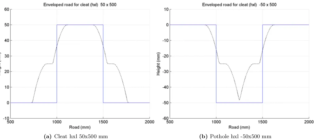
[image:13.595.48.552.65.291.2]

(a)Cleat hxl 50x500 mm (b) Pothole hxl -50x500 mm

Figure 2.7: The effect of tyre enveloping with a cleat and a pothole, representing the road profile (solid line) and the effecive road height (dashed line)

Something to take notice of is the fact that the envelopment of the road does not depend on the velocity of the truck, but of course the up and over time will decrease with an increasing velocity. This will lead to different responses of the components in the truck. The velocities which will be be used in this report are 10, 20, 30, 40 and 50 km/h. There are some other input values which can affect the shape of the enveloped road such as the diameter of the wheel and tyre stiffness, but standard values, as used within DAF, for all of these properties are used and therefore they are considered as a sort of black box.

After enveloping, the road model contains the longitudinal position and the corresponding effective road height. It is also possible to take the road slope and camber into account, which represents the change of the normal direction of the road’s surface w.r.t. the wheel’s centre. However for simplicity sake this was not used for the results in this report.

2.2.3 Cleat input

In order to investigate the response of the truck, a range of cleats will be used as input for the model. The height of the cleat will vary between -100 and 100 mm and the length from 0 to 1000 mm. In which a negative cleat height will represent a pothole.

(14)

2.2*TRUCK CONFIGURATION 7

From these 3D plots, some interesting things can be noticed;

• The shape of the enveloped road show great similarities for different road heights • Getting on the cleat has the same shape and slope as rolling off the cleat

• The maximal enveloped height is reached after about 150 mm this does not depend on the height of the cleat, this is about half of the footprint length of the tyre.

• The bottom of the pothole is not reached in figure 2.8b, this means that the tyre will not touch the ground for this length.

(a)Cleat with an constant heigth of 50 mm and a varying length (mm)

(b)Cleat with an constant length of 500 mm and a varying heigth (mm)

Figure 2.8: The effect of tyre enveloping

(a) Cleat with an constant height of 20 mm and a varying length (mm)

(b)Cleat with an constant height of 50 mm and a varying length (mm)

(c) Cleat with an constant height of 100 mm and a varying length (mm)

(15)

3. Truck response

Looking at the input of the model there are quite some variables to consider. These are velocity of the truck, cleat height and length, the different data points, the type of response (acceleration, force, displacements, springtravel). Several plots are shown in this chapter to get an initial feeling for all of these parameters.

3.1 Initial results

As already stated, symmetric load cases will be used for all simulations. This will reduce the amount of datapoints, since the left and the right side will show more or less the same response. There are some very small differences due to the fact that the truck itself is not completely symmetric, but these will not be taken into account. To start the analysis, the front axle will be investigated (the graphs are made from the data of the left side, but represent the entire front axis due to symmetry).

As already stated in the previous section about the cleat input, the shape of the enveloped cleat does not differ a lot when the cleat’s height is altered. The absolute values of the response will increase with an increasing cleat height, but the overall shape of the response stays the same. This effect will be discussed in more detail in section 3.2. The 3D surf plots in figure 3.3 are created for a cleat with a constant height of 50 mm and a variable length. On the other axis the response in the time domain is displayed. For every sub figure there are four graphs representing the different velocities of 20, 30, 40 and 50 km/h respectively.

Starting by comparing figure 3.1a and 3.1b with the input of the cleat from figure 2.9b. It seems to be that the initial moment of excitation is on different positions, but this can be explained since the excitation is in the time domain and the velocity is not the same. It can be noticed that the front axle will not reach the final displacement of 50 mm, but it will come close with increasing velocity. In general the triangular shape of the input can be recognized in all of the figures of 3.1a, from 3.1b it can be seen that the front axle will follow the shape of the enveloped road pretty well.

The graphs in figure 3.2a to 3.3b represent the acceleration of the axle and the damping force acting on the damper connected to the front axle respectively. These show quite some similarities when the overall shape is compared. It can be seen that the maximal peaks (negative and positive) seem to occur during the same circumstances. A relation is found for the up and over time of the tyre and these maxima and minima. Later on in this report, this effect will be investigated in more detail. However it can be said that for a higher velocity the maxima and minima shift towards a longer cleat.

These 3D plots give an interesting overall view of the influence of the length of the cleat, but it is still hard to identify and specify the occurrence of these peaks. Some general trends appear to be visible, but at this stage it is not possible to link peaks to specific events happening in the truck. However, it does show that the length of the cleat is of great influence on the response. In order to say something about the frequencies that arise during the excitation, a closer look will be taken at some of the interesting lengths of the cleat at a velocity of 20 km/h.

(16)

3.1*INITIAL RESULTS 9

(a)3D view front axle’s displacement response

[image:16.595.39.558.67.426.2]

(b)Altitude map of front axle’s displacement response

(17)

10 3.TRUCK RESPONSE

(a) 3D view front axle’s acceleration response

[image:17.595.35.556.51.762.2]

(b)Altitude map of front axle’s acceleration response

(18)

3.1*INITIAL RESULTS 11

(a) 3D view damping force from damper connected to the front axle at the left side

[image:18.595.39.552.70.753.2]

(b)Altitude map of the damping force of the damper connected to the front axle at the left side

(19)

12 3.TRUCK RESPONSE

3.2 2D response

Some interesting shapes and frequencies have come up from the 3D plots . Therefore, some 2D plots of several cleats will be investigated. Before looking at the cleats, a stepfunction will be used to give a preliminary feeling of the behaviour of the response.

3.2.1 Stepfunction

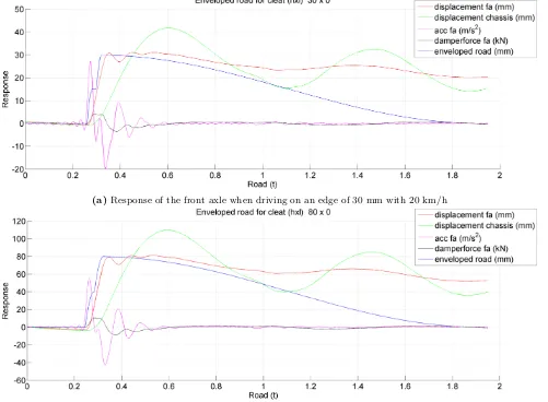
Before the cleat will be investigated a more simplified road input will be used to get a response. This will be a step function, thus more like riding on an edge and this will gradually leap towards zero again. This is basically the first part of the cleat. The results can be seen in figure 3.4. Heights of 30 and 80 mm are used to obtain the response. These figures will hold the enveloped road, the displacement of the Fa and the chassis, the acceleration of the Fa and the force acting on the damper. The velocity will be 20 km/h.

What you can see is that both graphs show a lot of similarities. Firstly looking at the displacements of the Fa and the chassis. The Fa has a small lag with respect to the enveloped road, this is caused by the stiffness of the tyre. Just after excitation it’s vibration has a frequency around 10 Hz and this corresponds to the Fa’s eigenfrequency. The chassis responds slower to the excitation, due to the dampers and springs between the Fa and the chassis. The eigenmode for which all components attached to the chassis start to bounce on the Fa, is around 1 Hz and this can be recognized in the displacement of the chassis as well.

(a) Response of the front axle when driving on an edge of 30 mm with 20 km/h

[image:19.595.51.552.378.746.2]

(b)Response of the front axle when driving on an edge of 80 mm with 20 km/h

(20)

3.2*2D RESPONSE 13

The acceleration response is more or less the same for both heights as well, the peaks are higher for the 80 mm case, but the overall response shape is the same. An important thing to consider is how an acceleration profile is formed. Acceleration is the second time derivative of the displacement and this roughly means: when the curvature of the displacement graph changes, the acceleration will change as well. Thus what you can see is when the displacement starts, the curvature of this displacement is the same for the 30 mm case as for the 80 mm case and therefore the acceleration response has the same shape in both cases. When the Fa has reached the top of the ramp, the curvature of the displacement changes again and the acceleration will become negative, this is the same for both graphs as well. The fact that the acceleration is higher for the 80 mm case can be explained by the fact that a larger distance has to be covered in the same time stamp.

3.2.2 2D plots of the cleat’s

As already mentioned, some typical lengths of the cleat will be investigated in the same manner as the stepfunction. To say something about the overall reaction of the Fa to a cleat. Some interesting lengths from the 3D plots will be investigated. These are 100, 450 and 900 mm. To make sure the cleat’s height does not greatly affect the behaviour this will be investigated as well for 30 and 80 mm. Thus in total six 2D plots will be used to identify the behaviour of the Fa for a velocity of 20 km/h. The graphs of the other velocities can be found in Appendix A, but these will not be discussed in more detail.

As can be seen in the legend, three responses are shown in figure 3.5. These are the displacement of the Fa and the chassis and the acceleration of the Fa. Starting with the displacement of the chassis (the green line), it can be seen in all figures that the displacement has a delay w.r.t. the input of the cleat just as with the stepfunction in the previous section. However, when one is looking at the amplitude of the response there are some large differences between a thin and a wide cleat. It could be said that in the case of a thin cleat, the chassis simply does not have the time to respond on the imposed displacement of the cleat. For wider cleats, the excitation is present for a longer time and thus has more influence on potential new obstacles. Besides the maximal amplitude caused by a higher cleat, there are almost no differences in the response caused by the different heights of the cleat.

The initial response of the Fa to the cleat is practically the same as to the response on the stepfunction, and this does not depend on the length of the cleat. Therefore it can be concluded that the initial response of the Fa is not affected by any future events. However, once the top of the enveloped road is reached large differences are present. For the 100 mm cleat it means that once the top is reached, the Fa immediately starts to go down again. For wider cleats some relaxation in the response can be noticed and this is directly related to the acceleration of the Fa.

(21)

14 3.TRUCK RESPONSE

(a) Response of the front axle for a height of 30 mm with a varying length with 20 km/h

[image:21.595.74.521.65.418.2]

(b)Response of the front axle for a height of 80 mm with a varying length with 20 km/h

(22)

3.3*CONCLUSION CLEAT RESPONSE 15

3.3 Conclusion cleat response

This chapter was started by investigating whether different cleat sizes would have different effects on the truck. In an early stage it was already quite clear that this was the case. By keeping the height constant and altering the length of a cleat, a bumpy landscape was found in the response. This was the case for displacement as well as acceleration, forces and spring travel. Thus it could be concluded, that a closer look was required to identify the behaviour of the truck to a certain height/length ratio of a cleat. Initially this was done by looking at a stepfunction, which only showed the response of driving on a cleat and not of it.

(23)

4. Sine Sweep

Up to this point, the emphasis was on a single excitation of the truck. The model ran over a cleat and afterwards the response was investigated. This was of great use to map the behaviour of the truck, but under normal use conditions most of the time it is not a single excitation that will cause problems. It is to this fact that more recurring bumps will be used for further research. By systematically reducing the distance between subsequent bumps an artificial road is created which covers a certain range of input frequencies. It is expected to provoke resonances in components of the truck when the input frequency of the subsequent bumps, is the same as the corresponding eigenfrequency. The study on the cleat in the previous chapter has given some insight in the response and dynamic behaviour of the truck, however due to the harsh edges of the cleat it is still not ideal to use these for real road test facilities. A form that is used more often is the sine shaped bump. This will be investigated in more detail in this chapter.

4.1 Sine shaped bump

[image:23.595.245.360.415.506.2]

Firstly a single bump has to be specified such that this bump can be used to create a recurring input signal for the model. The shape of the bump will be as a standard sine shaped speed bump, an example of these sort of speed bumps can be seen in figure 4.1. This will be modelled as using only the first half of a sine function as an input signal.

Figure 4.1: Example of a sine shaped speed bump [3]

The function to generate the sine as input is already available in the TricaT toolbox. Within this function there are some options of which you can chose to describe the sine. The first thing to consider is how much of the sine shape you will take, for example it is possible to take only the top of the sine. This will lead to different shaped bumps. It is the intention of this research to maximize the model’s output and with this in mind the shape will be looked at in more detail. From the study on tyre envelopment of road surfaces performed by Schmeitz [7] it was concluded that the response towards a vehicle is maximal when the change in road surface is perpendicular to the driving direction. This was the case with the cleat used in the previous chapter. The rest of the shape of the enveloped road depends on the other dimensions of the bump. Since the transition between the flat road and the bump will be the greatest in this case it can be concluded that the worst case scenario originates from a half sine and not just a part of it.

The other dimensions are the height (amplitude) and length (period) of the bump. It is advised by the DAF staff to take an height of 30 mm, since this is more or less a standard size in the industry. This leaves only the length of the bump for investigation. In order to tell something about the length, the envelopment behaviour of the tyre needs to be investigated in more detail.

(24)

4.1*SINE SHAPED BUMP 17 4.1.1 Sine envelopment

The same double cam tandem model will be used for the envelopment of the sine bump as was used for the cleat. Three examples of enveloped sine bumps are shown in figure 4.2. The difference in effective road profiles differ quite a lot, thus this means that envelopment for the sine bump is something to keep in mind. From the first plot it can be concluded that a relative thin bump will lead to two almost individual peaks. This is undesirable, since this will lead to an additional vibration in the input signal. From the other two plots it can be concluded that a wider bump leads to a profile which looks more like the original input since the maximum effective height will be higher. However, the additional widening w.r.t. the original bump of the enveloped road is almost the same for all three situations and it gives a widening of approximately 175 mm on both sides.

(a) Sine bump wxh 100x30 mm (b) Sine bump wxh 300x30 mm (c) Sine bump wxh 500x30 mm

Figure 4.2: Enveloped sine bumps with different widths, road profile (solid line) and the effecive road height (dashed line)

[image:24.595.47.551.243.402.2]

After some trial and error it came to notice that this widening of the enveloped road will be a crucial parameter since it has quite a large effect on the road. When the distance between two bumps reduces to approximately 350 mm, the end of the first bump will start to overlap the begin of the next bump. Resulting the neutral line to elevate w.r.t. the road. This effect is shown in figure 4.3 and is of course not desirable. The wider the bump, the sooner this effect start to kick in and thus a compromise has to be made. A thin bump will result in two individual peaks and a wide bump will cause the overlapping effect to kick in at an early stage.

(25)

18 4.SINE SWEEP

4.1.2 Operating frequency

Based on the information of the enveloped road alone, it is not possible to chose the optimal dimensions of the sine bump. When the truck drives with a certain velocity on the described road the distance between the subsequent bumps will cause a corresponding excitation frequency. The relevant operating frequency is between 1.1 (cabin roll) and 20 Hz. The frequency corresponding with a certain distance can be calculated with formula 4.1. Thus, when the truck drives 10 km/h (which is about the minimum velocity) the minimal distance between the first two bumps of the road has to be 2525 mm and the minimal distance between the last two bumps has to be 694 mm for a velocity of 50 km/h. The specific range of frequencies that will be covered at each velocity is shown in table 4.1. Based on this frequency overview, a velocity can be chosen when one wants to investigate a certain resonance frequency. ;

W avelength(mm) = V elocity (mm/s)

f requency (s−1₎ (4.1)

f irst gap= 10/3.6/1000

1.1 = 2525 mm (4.2)

last gap= 50/3.6/1000

20 = 694 mm (4.3)

Table 4.1: Frequency range corresponding to a velocity

Velocity (km/h) Frequency range (Hz)

10 1.1 - 4.0

20 2.2 - 8.0

30 3.3 - 12.0

40 4.4 - 16.0

50 5.5 - 20.0

Since the minimal distance between the last two bumps has to be at least 694 mm and the additional widening due to tyre enveloping is approximately 175 mm per side. The bump’s length will be 694−175·2 = 344 mmwhich will become 350 mm since this size is available on the market [1].

4.1.3 Number of bumps

Based on the size of the first and the last gap combined with the maximal length of the road which is 100 m (the maximal available test ground, provided by internal DAF engineers) and the fact that a constant distance reduction between the gaps is preferred, the total amount of bumps can be determined. By reducing the distance between the bumps with 30 mm per gap, 61 bumps are required to fill up the space of 100 m. Some trial and error has been used for different configurations but this setup gave the best results to obtain a smooth frequency transition.

4.1.4 Final sweep design

Formula 4.4 is used to determine the total amount of bumps based on the first and last gap distance, being 2525 and 694 mm respectively and a shortening for each gap with respect to the previous gap which is set at 30 mm. The total road lengthLtotal is found by summing all gap distances, and thus a

(26)

4.2*RESPONSE TO THE SWEEP 19

nbumps =

f irst gap−last gap

shortening (4.4)

Ltotal = nbumps

X

i=1

(f irst gap−shortening·nbumps) (4.5)

Figure 4.4: Enveloped sine sweep 350x30 mm with corresponding frequencies for 40 km/h, the blue line represents the input frequency for the subsequent bumps at that position (this uses the same values on the axis only in Hz)

4.2 Response to the sweep

As already stated in section 2.2.1 it is possible to obtain data from a lot of positions within the truck, but in order to keep things simple, only a few key components will be investigated. This involves the displacement and acceleration of the front and rear axle, the chassis (measured above the front axle) and the engine. Just as with the cleat, in this stage of the research only a symmetric load case is used as input. The velocity which gives the most interesting frequency range is 40 km/h (4.4-16 Hz), therefore this is used with the axles and the engine. The chassis reacts at a lower frequency, therefore 10 km/h is used to see the response of the chassis.

4.2.1 Front axle

From the list of eigenfrequencies available in the program Hyperview, it can be seen that the first eigenmode at which the front axle starts to bounce occurs at 9.41 Hz. Therefore it is expected to see a resonance in the response of the front axle at this frequency. As expected in the vicinity of the 10 Hz, resonance occurs as can be seen in figure 4.5. The displacement rises from approximately 15 to 22 mm and the acceleration increases from 45 to 85 m/s2_{. Just before the end of the sine sweep it}

can be noticed that the front axle tends to climb. The neutral position of the axle start to elevate, but the bumps do not overlap, so this means that the axle cannot follow the contour of the bumps.

4.2.2 Rear axle

(27)

20 4.SINE SWEEP

[image:27.595.44.559.125.418.2]

is a possibility that it is just the basic harmonic vibration of the 11 Hz vibration. since a frequency of approximately 11 Hz can be recognized in the acceleration plot. This would mean that the axle can come up and go down in the time between the next bump hits the tyre.

Figure 4.5: Front axle reponse for the sine sweep with corresponding frequencies with 40 km/h

[image:27.595.44.558.466.761.2]

(28)

4.2*RESPONSE TO THE SWEEP 21 4.2.3 Chassis

[image:28.595.39.558.249.548.2]

It is known that the chassis behaves a lot less high frequent and therefore this model will be driving with a velocity of 10 km/h on the sine sweep road. As already stated, the measure point of the chassis lies directly above the front axle on the left side of the truck, other points on the chassis will most likely show the same trend but can still have some deviations. The response can be seen in figure 4.7. The first eigenmode which corresponds to pitching of the cabin can be seen at approximately 1.3 Hz and this correlates with the 1.33 Hz from Hyperview for this mode. The second peak occurs around 1.8 Hz and this is also coupled to a pitching motion of the cabin. Therefore it can be stated that the motion of this part of the chassis is more or less directly coupled to the motion of the cabin and due to the springs and dampers between the axis any high frequent behaviour is filtered from the motion of the chassis.

Figure 4.7: Chassis response for the sine sweep with corresponding frequencies for 10 km/h

4.2.4 Engine

(29)

[image:29.595.42.556.69.367.2]

22 4.SINE SWEEP

Figure 4.8: Engine response for the sine sweep with corresponding frequencies for 40 km/h

4.3 Conclusion sine sweep

The goal of this chapter was to map the response of the truck when it was subjected to a sine sweep. Firstly the shape of an individual bump is determined and the next step was to create a road surface with these bumps which could cover a range of interesting input frequencies for the truck. It depends on the velocity of the truck which frequency range is touched. It was provided that the maximum length of the sine sweep should not be more than 100 m and this resulted in a road with 61 sine shaped bumps.

(30)

5. Theoretical evaluation

The results from the sine sweep have proven that it is possible to provoke resonance in a component. This will occur when the drive conditions match the eigenfrequency of this component, which is a combination of driving velocity, the distance between the bumps and a continuous input signal. Due to the fact that resonances can be present, the question arose whether this could cause problems during real world drive conditions. This chapter will take a closer look at the phenomena which causes resonance for damped and undamped systems and how this affects some components.

5.1 Resonance

From the results obtained with the sine sweep it is clear to see that under specific road conditions it is possible to provoke resonance. However, the time (and thus the amount of bumps) in which the maximum peak has been reached differs for damped and undamped components. Therefore it is interesting to investigate this observation in more detail.

If a resonance occurs in a mechanical system it can be very harmful and can lead to eventual failure of the system. It is important to identify under which road conditions resonance may occur and then to determine what steps to take to prevent it from occurring. The amplitude plot in figure 5.1 shows that adding damping can significantly reduce the magnitude of the vibration. This figure shows the ratio between the input frequency ω divided by the natural frequency ωn and the corresponding

[image:30.595.146.446.432.637.2]

amplification ratio of the system.

Figure 5.1: the frequency response of the system [8]

It can be seen that when the input frequency approaches the natural frequency (the ratio becomes 1) the amplification ratio starts to grow and depending on the amount of damping, this ratio can become significantly higher. It can be seen that when an harmonic input is applied to an undamped system at a frequency corresponding to it’s natural frequency, the magnitude of the response is infinite and this is the moment when resonance start to take place. This phenomena is shown in figure 5.2, it shows an increase of amplitude and it will keep increasing until the system fails or when the movability comes to a maximum.

(31)

24 5.THEORETICAL EVALUATION

Figure 5.2: Increasing amplitude of a system excited in it’s eigenfrequency

Of course, a situation where the amplitude gets infinitely large can never occur in a real life system since some damping such as rayleigh damping is always present in actual systems. Nevertheless this concept is of practical importance since a large response is acquired whenever an harmonic exciting force is near the natural frequency of an undamped system.

Resonance is simple to understand if the spring and mass are considered as energy storage elements. In which the mass stores kinetic and the spring potential energy. The mass and spring have no external forces acting on them and therefore they transfer energy back and forth at a rate equal to the natural frequency. In other words, to efficiently pump energy into the mass and spring it requires the energy source to feed energy at a rate equal to the natural frequency. The force applied does not need to be high to get large motions, but it must just add energy to the system [8].

When a damper is included an element is introduced which dissipates energy instead of storage. Damping force is proportional to velocity, the greater the motion, the more energy is dissipated by the damper. Therefore there is a point when the energy dissipated by the damper equals the energy added by the harmonic excitation. At this point, the system has reached its maximum amplitude and will continue to vibrate at this level as long as the applied harmonic force stays the same. This also applies to internal damping, eventually an equilibrium will be reached. This effect is displayed in figure 5.3 a and b, in which the excitation is scaled to it’s maximum excitation. It can be seen that lesser damping will lead to a higher amplitude of the response. Besides having a higher maximum it also needs more cycles to reach the steady state solution. An indication for the amount of cycles which are required to obtain 95% of the maximum amplitude is shown in figure 5.4.

[image:31.595.204.396.72.239.2]

(a)Damped resonance envelopement (b)Damped resonance response for increasing damping

(32)

5.1*RESONANCE 25

Figure 5.4: Number of cycles required to reach 95% of the steady state vibration [4]

The maximal amplitude and the amount of required cycles to obtain this maximum is directly related to the amount of damping. The enveloped shape of the growth of the amplitude is given by formula 5.1 [4]. This formula shows that the maximum is related to the factor 1/2ζ. However, something which gets little attention in literature is the relation between the amplification factor and the amount of damping for a given amount of cycles. To map this relation, formula 5.1 is used for different amount of viscous dampingζ. A contour plot of the results can be seen in figure 5.5. This gives an indication for the amplification factor for a given amount of cycles, and based on this graph it is possible to choose whether damping is preferred in a component. A part of the decision to add damping or not is the feasibility of the recurring amount of bumps in the road profile. However, a real life road probability study is not part of this research.

u(t) = 1 2ζ(e

−ζωt₋

1) (5.1)

(33)

[image:33.595.44.560.68.428.2]

Figure 5.5: The influance of damping on the amplification factor, in a resonant system, shown for different amounts of damping (ζ) plotted against the number of oscillation cycles.

5.2 Quarter car model

One of the most used models of a vehicle suspension sytem is the quarter car model [6] as displayed in figure 5.6. It is used for vertical vibration of a vehicle. This model consists of two solid massesms

and mu which stands for the sprung and unsprung masses. The sprung mass ms represents 1/4 of

the body of the vehicle and the unsprung massmu represents one wheel and a part of the axis of the

vehicle (a quarter of the car). The wheel is connected to the road with a springku which represents

the tyre stiffness and the suspension of the car is modelled as a spring ks and damper cs.

[image:33.595.239.355.610.758.2]

(34)

5.3*RESONANCE IN THE COMPONENTS 27

The equations of motion (Eom) of this model are given in equations 5.2 and 5.3.

msx¨s+cs( ˙xs−x˙u) +ks(xs−xu) = 0 (5.2) mux¨u+cs( ˙xu−x˙s) + (ku+ks)xu−ksxs=kuy (5.3)

which can be expressed in a matrix vector form as:

ms 0

0 mu

¨ xs ¨ xu +

cs −cs

−cs cs

˙

xs

˙

xu

ks −ks

−ks ks+ku xs xu = 0

kuy

(5.4)

This is of the form as in formula 5.5 in which [M] is the mass matrix, [C] is the damping matrix, [K] is the stiffness matrix and {F(t)} is the external force vector.

[M]{¨x}+ [C]{x˙}+ [K]{x}={F(t)} (5.5)

A quarter car model does not take any internal dampers, geometric effects or internal vibrations into account. It also does not offer a possibility to study longitudinal and lateral vibration, but since only symmetric load cases were used this will not influence the results for this report. Looking at the quarter car model, the spring ku which represents the tyre stiffness can be seen as a sort of filter.

Excitements from the road are being transferred to the unsprung mass with a small delay, but in general all energy is directly transferred. This model will be used as a basis for the evaluation of the upcoming simulations.

5.3 Resonance in the components

The quarter car model has reduced a complex system of dampers, springs, truck components and their internal connections to a simple mass spring damper system. With this simplified model it is possible to get a feeling for the behaviour of some of the components. In this model the sprung mass represents a quarter of the weight of the components in the truck. some of these components, such as the engine, are connected to the chassis with dampers, but others such as the fuel tank are not. Therefore it is interesting to see whether it is possible to provoke resonance, as was shown with the sine sweep, in order to reach the maximum excitation in these components as described in section 5.1. The Eom of the quarter car model are of interest when the response of these masses were of required, but for this study, only the global representation is used.

From the sine sweep it became clear that it is possible to provoke resonance, but it is still not clear whether it would actually happen under real life road conditions. Therefore two components will be investigated, the rear axis represented by the sprung mass and the fuel tank which can be seen as an extra mass connected to the sprung mass with nothing but springs since it is only subjected to internal damping and damping from surrounding components.

The input frequencies which result in resonance can be found from the sine sweep. Two subsequent peaks from the response were used to calculate the frequency which gave the highest output for the axle and the fuel tank. And after some fine-tuning the highest amplitudes were found at an input frequency of 11.36 and 10.20 Hz respectively. The bumps which were used for this simulation were the same as for the sine sweep.

(35)

5.3.1 Resonance in the Rear Axle

From the model in Hyperview it was found that the first eigenfrequency of the rear axle was 11.28 Hz. However from the sinesweep followed that the a maximal excitation was obtained at 11.20 Hz. These were both tested and the second frequency gave a higher response, thus this was used in the analyses. This resulted in a bump distance of 1222 mm at a velocity of 50 km/h. 30 bumps were used to show that a steady state solution was reached. The maximal steady state acceleration amplitude of 195.8

[image:35.595.94.506.188.505.2]

m/s2 was reached after only 6 cycles. The results can be seen in figure 5.7.

Figure 5.7: Rear axle excited at a frequency of 11.36 Hz at 50 km/h

5.3.2 Resonance in right Fuel Tank

The displacement and acceleration plots of the fuel tank are a little harder to interpret. This comes from the fact that all values are absolute values, meaning that when the entire truck moves up and down, this will affect the individual components as well (this was also the case for the axis, but these experience little interference from other parts). The eigenfrequency of the fuel tank was found at 10.20 Hz from the sine sweep. At first this frequency seemed to be strange, since the model in Hyperview gave an eigenfrequency at 9.03 Hz. This can probably be explained by the fact that the energy must be transferred through the rear axle and the chassis towards the fuel tank. The rear axle’s eigenfrequency is around 11 Hz, thus when approaching this frequency it leads to an increase of amplitude, and thus an increase of transferred energy. Apparently, the combination of energy transferred by the rear axle and the maximal resonance of the fuel tank occurs at 10.20 Hz. This also means that the maximal theoretical amplitude, when excited exactly in it’s eigenfrequency, will not be reached, because the excitation force is smaller when the rear axle is not resonating. At a velocity of 50 km/h this resulted in a gap distance of 1361 mm and once again 30 bumps were used to show that a steady state was reached. The results can be seen in figure 5.8.

(36)

5.3*RESONANCE IN THE COMPONENTS 29

1 Hz, this can be recognized as the overall displacement of the chassis. The acceleration graph gives a more clear image of the resonance. It shows a gradually increase in amplitude, something that can be recognized as a response with a small amount of damping. The maximal amplitude of 31.8 m/s2

is reached after 16 cycles.

Figure 5.8: Fuel tank excited at a frequency of 10.20 Hz

5.3.3 Velocity alternation

[image:36.595.76.520.134.475.2]

By using a different velocity on the same track, it will change the input frequency of the bumps. Since the input frequency changes this will also affect the response. At 50 km/h the rear axle and the Fuel tank were excited in their eigenfrequency and by changing the velocity, this is no longer the case. The results corresponding to a velocity of 40, 50 and 60 km/h can be seen in table 5.1.

Table 5.1: Frequencies corresponding to alternative velocities with the maximum acc amplitude and the number of cycles required to reach this maximum

Rear Axle Fuel Tank

Velocity (km/h)

Frequency (Hz)

Max Amplitude (m/s2₎

Cycles to max

Frequency FT (Hz)

Max Amplitude (m/s2₎

Cycles to max

40 9.09 88.9 2 8.16 20.9 5

50 11.36 195.8 6 10.20 31.8 16

60 13.64 150.0 3 12.25 26.6 5

(37)

amplification factor. A thing to notice though, is the number required cycles to reach the maximum amplitude. These are significantly lower when the system is not exerted in it’s eigenfrequency. How-ever, further research should be done whether these accelerations of the fuel tank are caused by the total displacement of the truck or if the tank is actually vibrating with respect to the chassis.

5.3.4 Gaps in the input

[image:37.595.76.520.330.665.2]

Now that it is shown that it is possible to generate resonance in the components another aspect needs to be investigated. This is the effect of a larger gap between two subsequent bumps. Therefore two gaps of 5000 mm are placed after the fifth and fifteenth bump. The results can be seen in figures 5.9 and 5.10. These graphs show quite an interesting response, since they both start oscillating at their eigenfrequency and show an increase of amplitude just as seen before. However, the axle needs less oscillations to reach the maximum and therefore the axle is able to reach the maximum within the relative short continuous input. At the other hand the damping within the suspension leads to a significant decay in amplitude during the absence of the bumps.

Figure 5.9: Rear axle with interverance in the input signal

(38)

[image:38.595.77.518.66.410.2]

5.4*CONCLUSION THEORETICAL APPROACH 31

Figure 5.10: Fuel tank with interverance in the input signal

5.4 Conclusion theoretical approach

From these results it can be concluded that a poorly damped component will probably never reach the maximum excitation amplitude under real life road conditions (According to DAF a minimum value ofζ = 0.025 is always present in a truck) due to internal hysteresis. There are simply to many factors who all need to be perfectly converged. These are velocity, corresponding eigenfrequency, constant harmonic input and probably the most crucial thing is the fact that there can hardly be any interference in this input. In the case of the Fuel tank, it means that at least 16 bumps have to be perfectly aligned for a specific velocity and this is just to much of a coincidence that it most likely will never occur during normal drive conditions. Even if there would be a situation at which this maximum is reached it would be to rare to take this into account in the design of the truck. However, it has been shown that the amplification factor can highly vary for poorly damped and slightly damped systems.

(39)

6. Conclusion and recommendations

6.1 Conclusion

This study was set out to identify vehicle response with computed standardized tracks. The motivation to investigate specific road truck interaction came from newly measured road data from Brazil. The road conditions in Brazil differ quite a lot compared to the roads in Europe. These roads have a large variety of bumps and holes which have a large impact on the truck’s lifespan. DAF’s proving ground in St Oedenrode already provided a large amount of data, but this still lacks the highest peaks as measured in Brazil. Therefore this study was used to map the truck’s behaviour to artificial road profiles and evaluate the virtual response in order to define possible alternative road inputs.

With the use of TricaT, this research started by looking for differences in the truck’s response for various cleat sizes. In order to limit the amount of output, only symmetric road input was used. By keeping the cleat’s height constant and altering the length a large variety of output was obtained. This showed large differences in displacement, acceleration, forces and spring travel on several parts of the truck. From these results it could be concluded, that it was necessarily to investigate the truck’s behaviour in more detail. This was done by taking interesting height/length ratio’s of a cleat and analyse these individually. These analyses resulted in the conclusion that the overall shape of the response profiles do not differ by alternating cleat heights, this only changed the absolute values. By changing the length of the cleat it was shown that a maximal output could be provoked when the combination of driving velocity and the length of the cleat (up and over time) matched the eigenfrequency of a component.

It has been shown that specific road conditions lead to a maximum in the response. This induced the question, whether it was possible use this maximum to subject the truck to a sine sweep with speed bumps to provoke resonance. The dimensions of the sine shaped speed bump were set at 30 mm heigh and 350 mm long. These were found to be the most useful dimensions after enveloping. In total 61 speed bumps with a decreasing subsequent distance of 30 mm were used, these covered a total road profile of 100 m. By looking at the eigenfrequencies and corresponding eigenmodes, it was possible to forecast and provoke resonance for several components. However, when some of the internal components such as the engine and the fuel tanks were investigated, the identification of the eigenfrequencies became more complicated. The simulations showed several peaks in the response but these could not be coupled directly to their eigenmodes.

In the final stage of this research the previously found insights were coupled to the theory about mass spring damper systems. This was used to see whether resonances would actually cause problems in some of the components. This resulted in the conclusion that under real life road conditions a poorly damped component, such as a fuel tank, will probably never reach the maximum excitation amplitude caused by resonance. However, it has been shown that the amplification factor highly varies for poorly and minor damped systems. For damped components such as the axis, the cabin and the engine, resonance is something to take into account. They need much less cycles to reach the maximal excitation and therefore the possibility that an absolute maximum is reached by resonance is a lot higher.

This research has led to the identification of the truck’s response for several road inputs. It has identified some of the most crucial road conditions and eventually it has been shown how resonance could affect different components. These results can be used in further research on road simulation, such that data from real life road conditions can be coupled to virtual test grounds.

(40)

6.2*RECOMMENDATIONS 33

6.2 Recommendations

This research has given initial results on truck road behaviour, but there are still some fields in which further research could be done. This would lead to an even further understanding of the truck’s response in real life road conditions. The recommendations are stated below:

• Some components such as the axis are elaborated in high detail in this report, but there are many more components in the truck whom also could be tested for phenomena such as resonance.

• This study started using not only cleats, but also potholes. Due to a lack of time, potholes were not discussed any further, but these could give some interesting results when they are combined with the speedbumps. Currently only upward excitation is used in the form of a speedbump, but when the downward motion was strengthened by driving into a hole this could potentially feed the displacement of the components even further.

• The model in TricaT which is used for the envelopment of the road profile, does not make use of the change of slope when driving on or of an obstacle. For larger objects this change in slope leads to a changing normal vector and thus it has an effect on the overall force and moment balances. This will not have an effect on the displacement of the truck, but it could slightly affect the forces on several members.

• All acceleration and displacement plots, as shown in this report, are absolute values, thus this includes the overall displacement of the truck. If it is possible to uncouple the components in order to get relative displacement and acceleration data, this could show the real severity due to resonance.

• An assumption about the occurrence of real life road bumps was made, but in order to fully support this statement a probability study on this topic should be done. This could give insights in real life occurrence of these bumps.

(41)

Bibliography

[1] alibaba.com. 350mm wide abs plastic speed bump. http://www.alibaba.com/product-detail/ 350mm-wide-ABS-plastic-speed-bump_60465164185.html?spm=a2700.7724838.0.0.nsDzP5. [cited May 27 2016].

[2] M.A.F. Backx. Modelling the pothole road, DC 2013.056. Eindhoven University of Technology, Internal Report, 2013.

[3] bcsiteservice. Rubber speed bump. https://www.bcsiteservice.com/product/ rubber-speed-bump/. [cited May 25 2016].

[4] J. R. Clough. Dynamics of structures, pages 40–48. Computers and Structures Inc., Berkeley, CA 94704, 1995.

[5] Besselink I.J.M. Eindhoven University of Technology, dept. Mechanical Engineering, section Dy-namics & Control, Advanced Vehicle DyDy-namics. Lecture notes, 2013.

[6] Reza N. Jazar. Quarter Car, pages 931–975. Springer US, Boston, MA, 2008.

[7] A.J.C. Schmeitz. A Semi-empirical Three-dimensional Model of the Pneumatic Tyre Rolling Over Arbitrarily Uneven Road Surfaces. Delft University of Technology, 2004.

[8] Unknown. Vibration. https://en.wikipedia.org/wiki/Vibration. [cited June 14 2016].

(42)

(43)

36 A.FA CLEAT RESPONSE 30, 40 50 KM/H

A. Fa Cleat response 30, 40 50 km/h

(a)Response of the front axle for a lenght of 100 mm with 30 km/h

(b) Response of the front axle for a lenght of 450 mm with 30 km/h

[image:43.595.89.508.112.793.2]

(c) Response of the front axle for a lenght of 900 mm with 30 km/h

(44)

37

[image:44.595.73.524.41.774.2]

(45)

38 A.FA CLEAT RESPONSE 30, 40 50 KM/H

[image:45.595.75.523.66.756.2]

(46)

(47)

40 B.INFLUANCE SPEED ALTERNATION TO RESONANCE

B. Influance speed alternation to resonance

(a)Response of the rear axle with constant distance between bumps with 40 km/h

[image:47.595.103.496.109.756.2]

(b) Response of the rear axle with constant distance between bumps with 60 km/h

(48)

41

(a)Response of the right fuel tank with constant distance between bumps with 40 km/h

[image:48.595.103.493.72.687.2]

(b) Response of the right fuel tank with constant distance between bumps with 60 km/h

Vehicle response on standardized tracks

University of Twente

INTERNSHIP AT DAF TRUCKS N.V. APRIL-JULY 2016

Vehicle response on standardized tracks

Vehicle response on standardized tracks

Preface

Abstract

Contents

Nomenclature

1.

Introduction

1.1

Motivation and background

1.2

Goal of the study

1.3

Overview of the report

2.

The simulation model

2.1

Software

2.2

Truck configuration

3.

Truck response

3.1

Initial results

3.2

2D response

3.3

Conclusion cleat response

4.

Sine Sweep

4.1

Sine shaped bump

4.2

Response to the sweep

4.3

Conclusion sine sweep

5.

Theoretical evaluation

5.1

Resonance

5.2

Quarter car model

5.3

Resonance in the components

5.4

Conclusion theoretical approach

6.

Conclusion and recommendations

6.1

Conclusion

6.2

Recommendations

Bibliography

A.

Fa Cleat response 30, 40 50 km/h

B.

Influance speed alternation to resonance