Desalination on Microscale The Effect of Salt Concentration on the Desalination Performance of a Microfluidic Device

1

Desalination on Microscale

The Effect of Salt Concentration on

the Desalination Performance of a Microfluidic Device

Evelien C. Kamphuis

Bachelor’s Thesis

July 2017

Abstract

In order to increase the fresh water supply on earth, electrodialysis (ED) is widely used as desalination technology for generating potable water from brackish water. To give a better understanding of this principle, experiments at microscale have been performed in a previous proof-of-concept study at the University of Twente. The used microfluidic device, with hydrogels that mimic the membrane stacks of an ED device, has shown promising results at low concentrated NaCl-solutions.

Contents

1 Introduction 1

1.1 Motivation . . . 1

1.2 Scope . . . 1

1.3 Report structure . . . 1

2 Theoretical framework 2 2.1 Electrodialysis . . . 2

2.2 Ion Concentration Polarisation . . . 3

2.3 Current density . . . 4

2.4 Current regimes . . . 5

3 Experimental plan 6 3.1 Experimental Theory . . . 6

3.2 Methods & Measurements . . . 9

3.3 Hypotheses . . . 12

4 Results & Discussion 13 4.1 Experimental results . . . 13

4.2 Modelling results . . . 17

4.3 Discussion of Methods & Measurements . . . 20

5 Conclusion 21

6 Recommendations 22

1

|

Introduction

1.1 Motivation

The scarcity of water gives a major challenge for securing enough fresh water for human, environmental, social and economic demands. To generate potable water, a possibility is to remove salts from seawater or brackish water, also called desalination. This technique is of vital importance in order to increase fresh water supply. A widely used approach for desalination is electrodialysis (ED). To better understand the effects of solutions with different salt concentrations on the desalination performance of larger-scale ED, a microfluidic device with hydrogels as functioning membranes can be used. In a previous research at the University of Twente, a proof-of-concept desalination on a microfluidic device has been tested with low salt concentrations, giving promising results in order to better understand desalination on larger scale [1]. In this research, these devices are tested at higher salt concentrations to investigate the compatibility of hydrogels at these elevated concentrations.

1.2 Scope

The scope of this bachelor assignment is to characterise the effect of different inlet salt concentrations on the desalination performance of a microfluidic device. A closer look will be taken to the following measurable performance parameters: the salt removal efficiency and the current efficiency. In the earlier mentioned proof-of-concept study, the physics of desalination on a microfluidic device has already been performed with low concentration, below 1 mM [1]. In the experiments of this work the same set-up will be used, but experiments with higher concentrated salt solutions (1mM to 10 mM) will be performed. With higher salt concentrated solutions, the amount of salts will be closer to the amount of salts in less ideal brine solutions. In other words the concentrated solutions would be relatively closer to the salt concentrations of brackish water. If the desalination performance will not deteriorate with the use of higher concentrated salt solutions, this will contribute in fundamental research of desalination of brackish water, where hydrogel stacks mimic the ion exchange membranes of an ED stack.

1.3 Report structure

2

|

Theoretical framework

The background theory of ion-exchange through a membrane system will be explained. First, an introduction will be presented of the main principle: electrodialysis. Followed by information about ion concentration polarisation, current density and the different current regimes.

2.1 Electrodialysis

Electrodialysis (ED) can be used as a technique for the desalination of brackish water sources. A schematic overview of this ED process is given in Figure 2.1. It is a separation process technology, where a feed stream flows through (spacer) channels which separate a series of alternating cation and anion exchange membranes. These membranes are of opposite charge in comparison with the ions that will pass them. The exclusion of co-ions, ions with the same charge as the membrane, is called the Donnan exclusion. The electroneutrality in the membrane and the solution is disturbed, because of the fact that ions carry a charge [2]. In addition, an electric field is applied over the membrane stacks. Ions are moving in the electric field towards the electrode with opposite charge, but are selectively blocked by the membranes. When this process of ion exchange has taken place over a certain amount of membrane area, the outflows will be split into depleted and enriched salt streams [3]. An advantage of ED is that it is easy to scale and therefore it is very useful for small-scale desalination experiments. In this way, fundamentals of ion transport phenomena near membranes can be investigated at microscale.

Figure 2.1: Principle of electrodialysis where the driving force is the electrical potential [4]. CEM and AEM stands for cation and anion exchange membranes, respectively.

In the ideal case, the cation exchange membranes will only conduct the cations while the anion exchange membranes will only conduct the anions, due to ion selectivity. If a membrane is fully permselective, the counter-ions will carry all the current in the membrane. The transport number of this counter-ion equals one [2]. The transport number (ti) is defined as the current that is carried

2.2 Ion Concentration Polarisation

For the ion transport in ED-systems, three ion fluxes are involved: the convective flux as a result of convection perpendicular to the membrane, a diffusive flux resulting from a concentration gradient and a migrative flux in the electric field [2, 4]. These three parts are visible in Equation (2.2.1).

Ji=vCi+Di

dCi

d x −

ziF CiDi

RT

dφ

d x (2.2.1)

In this equation Jirepresents the flux of a specific ioni, and v and Cirepresent the convective transport

velocity and concentration, respectively. Di is the diffusion coefficient of the specific component,

which is multiplied by the derivative of the concentration in the horizontal x-direction in order to gain the diffusive flux. ziindicates the valence of the component, F and R represent the Faraday and gas

constant, respectively, followed by the Temperature (T). To get the migrative flux, this whole term is multiplied by the derivative of the electrical potential over the x-direction. In comparison with the other fluxes, the convective flux can be neglected, because the membranes are non-porous and there is thus no convective flow through the membranes. In this way, Equation (2.2.1) becomes similar as the Nernst-Planck equation, where ion transport over ion exchange membranes are only depending on two driving forces: the concentration and the electrical potential.

Ion Concentration Polarisation (ICP) is a phenomenon that limits the ion-exchange process through the membranes, which negatively influences the performance of an ED system because of the increasing electrical resistance of the solution [5]. It is desirable to work at the highest current density, to have a maximum ion flux over the membranes, but this becomes difficult due to ICP [2]. The reason of this phenomenon is the difference in the earlier mentioned transport numbers of the solution and the membrane. In the solution it can be assumed that tifor the cations and anions are roughly similar,

but in the permselective membrane the current is largely carried by the counter ion. Due to this, a boundary layer is formed at the interfaces of each side of the membrane. Between the desalting membrane surface and the (diluate) solution, the salt concentration will be relatively more depleted in the boundary layer. On the other side where the solution is enriched with ions, the concentration in the boundary layer will be relatively increased. This concentration profile is presented in a simple outline in Figure 2.2. Cbindicates the solution or bulk concentration and Cmindicates the concentration at the membrane surface. Only the ion fluxes on the left side are presented. Where Jd i f₊ and Jmi g₊ represents respectively the driving force of diffusion and migration of the positive counter-ion, which is visa verse also valid for the negative co-ins. Furthermore, electroneutrality over the whole system is assumed.

This ICP phenomenon will lead to a voltage drop, also called ‘internal resistance’, across the electrolyte [6]. The appearance of this transition is generally observable in current-voltage curves (IV-curves). At a certain potential the limiting current is reached, due to ion concentration polarisation. This limiting current will further be explained in Section 2.3. To reduce ion concentration polarisation, the flow rate could be increased in order to promote turbulence around the membranes, which will result in better mixing and a reduced thickness of the boundary layer.

2.3 Current density

In the membrane, the driving diffusional force can be neglected [2]. This is because the charge concentration in the membrane is relatively large in comparison with that of the solution. As a result, only the migrative part of Equation (2.2.1) is assumed to be valid in the membrane. With this assumption, the ratio between the positive and the negative ion flux (J₊and J₋) is equal to the ratio of the ion transport numbers (¯t₊and ¯t₋) in the membrane:

J+ J−=

−t¯ 1−t¯+

(2.3.1)

For this equation, it is assumed that the electrolyte solution only contains univalent ions (C₊= C₋= C). The sign in Equation (2.3.1) is negative, because the fluxes are vectors and have an opposite direction from each other, while the transport numbers are always taken positive.

In the boundary layer the diffusion flux does play an important role. So, the flux for both ions which has already been described in Equation (2.2.1) (without the convective part) is valid. To determine the current density, a steady state situation is considered. In this case, the fluxes in the membrane equal the fluxes in the boundary layer. Where the ionic diffusion coefficients from Equation (2.2.1) can be rewritten to the diffusion coefficient of the electrolyte D, see Equation (2.3.2). In the solution the ratio of the ionic diffusion coefficients (D₊and D₋) is equal to the ratio of the solution transport numbers (t₊and t₋).

D= 2D+D−

D₊+D₋=2D+(1−t+) (2.3.2)

When all above mentioned equations are combined, the current density (i) can be determined with the help of Faraday’s law, whereiequals the Faraday constant times the difference in ionic fluxes. The rewritten equation, which is also integrated over the boundary layer thickness (δ), is as follows:

i= _¯F D t₊−t₊

Cb−Cm

δ (2.3.3)

In Equation (2.3.3)F represents the Faraday constant, D is the diffusion coefficient, ¯t₊ andt₊are respectively the positive charged transport numbers of the membrane and the solution and Cmand Cb are respectively the concentrations at the membrane surface and in the solution. In this equation, the following assumptions are made: the transport numbers and the diffusion coefficient are constant over x. In this way, the concentration gradient in the boundary is also constant. Wheniis increased, the difference between Cmand Cb becomes larger, because Cmdecreases. At a certaini, Cmwill reach zero. At this point, the limiting current density (il i m) is reached. This transition in current behaviour

2.4 Current regimes

The behaviour of the current in IV curves can be distinguished into three current regimes, see Figure 2.3. These regimes will shortly be explained.

Figure 2.3: Conceptual representation of the relation between the current through a membrane and the corresponding voltage drop over the membrane and their boundary layers [7].

Ohmic regime

In the first regime, the Ohmic regime, the current density is low. There is a positive linear relation between the current and the voltage drop over the membrane [7, 8]. In this case Ohm’s law is valid, which allows that the effective resistance of the membrane system can be deduced from the slope of the IV-curve. As mentioned in Section 2.3, there is no depletion or ion enriched layer formed on each side of the interface of the hydrogel yet. This is also visible in Figure 2.3. The curve has the largest slope in the Ohmic regime. With Ohm’s law is derived that the resistance is low in this regime, as follows that the conductivity over the system is high. Hence, in this regime the current efficiency is most ideal.

Limiting regime

In this regime the limiting current density is reached, which has already been explained previously. The limiting regime is attained when the current does not increase with the electric field strength due to ion concentration polarisation. As a result, the process efficiency will be limited [2]. This regime is shown in Figure 2.3 as a flattened plateau.

Over-limiting regime

3

|

Experimental plan

This part of the report is split in experimental theory and an overview of the methods and measure-ments.

3.1 Experimental Theory

Microfluidic device

In the experiments, charged hydrogels will be used as anion and cation membrane interfaces, which simulate the membranes in ED stacks [1]. In Figure 3.1 a schematic representation of this micro chip is given.

A problem that could be faced using membrane stacks at micro scale, is the challenging fabrication, because of robustness and difficulties in consistency [1]. This could for example lead to liquid leakage. Because of these reasons, hydrogels give a good alternative for the membrane stacks. It can be incor-porated relatively easy in the microfluidic device and it makes the device less expensive. Furthermore, hydrogels provide good study towards the hydrodynamic and ion transport phenomena in microfluidic devices. To place the hydrogels in the device, a capillary line pinning technique is used for controllable patterning.

(a) Schematic top view (b) Zoomed top view with ion exchange principle

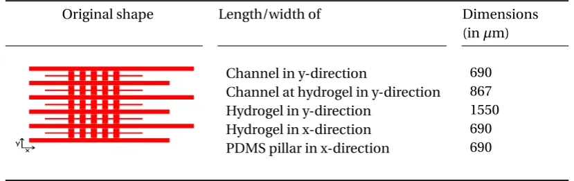
For the experiments, the original type of the microchip is used. It contains six microchannels, each with a separate inflow. The dimensions are given in Table 3.1.

Table 3.1: Schematic representation of micro chip with dimensions.

Original shape Length/width of Dimensions

(inµm)

Channel in y-direction

Channel at hydrogel in y-direction Hydrogel in y-direction

Hydrogel in x-direction PDMS pillar in x-direction

690 867 1550 690 690

The microchip consists of hydrogel pillars and capillary barriers [1]. The components of the hydrogel pillars are made of polydimethylsiloxane (PDMS) and are interlinked by six microchannels. To create a charge selective interface in the AEHs and CEHs, the charged monomers [2-(methacryloxyloxy)ethyl]tri-methylammonium chloride (METC) and 3-sulfopropyl acrylate potassium salt (SPAP) are used. In order to form METC and SPAP polymers, the monomers are photo-polymerised with acrylamide, N,N’-bis(2-hydroxyethyl)-ethylenediamine (bis) and free radicals yielded by 2,2-dimethoxy-2-phenylaceto-phenone (DMPA). Advantages of these polymers are that they have a high swelling degree, the hydrogels can absorb a high water content, and they have a good hydrolytic stability, which provides charge-based separations in micro chips. Moreover, the polymers have permanent positive and negative charge densities, which are independent in a large pH range (pH of 2-12). However, the permselectivity of the AEHs and CEHs have a moderate percentage of respectively 29 and 26%, due to the capability of absorbing large amounts of water. The moderate permselectivity of the hydrogels will negatively influence the desalination and current efficiency. How to determine these efficiency values, will later on be discussed in this section.

Salt solutions

To handle fresh water supply by electrodialysis, as mentioned in the ‘Introduction’, a microfluidic device is used to better understand the concept on smaller scale. In order to use the microfluidic device in the experiments, salt solutions are used to better mimic the concentrations of brackish water. The classification of water with associated dissolved salts are given in Table 3.2. In the experiments, lower concentrations will be researched (0.1 to 5.0 mM, equal to 6 to 292 ppm) to determine if the device works in this concentration range. Brackish water consists of different types of salts. However, due to the short period of time for this bachelor assignment, no differentiation will be used in the solutions. The experiments will be limited to different concentrated NaCl-solutions.

Table 3.2: Classification of water based on concentration of salts [10].

Designation Total dissolved salts (ppm)

Fresh water <500

Slightly brackish 500 - 1000

Brackish 1000 - 2000

Moderately saline 2000 - 5000

Saline 5000 - 10000

Highly saline 10000 - 35000

Brine >35000

Efficiency determination

After performing the experiments, the parameters current efficiency and salt removal efficiency can be determined to see whether or not the desalination performance will deteriorate.

With the current efficiency (CE) the optimum range of applicability of an ED cell can be determined [11]. Besides this, the total area that is required for the desalination can be subtracted from this efficiency. CE describes how well ions are transported over the membranes when a certain current is applied. In Equation (3.1.1) the determination of CE is given over one cell pair, in which the difference between the inflowing ions in the channel per second and the outflowing ions in the desalinated channel per second is divided by the total ion transport per second.

C E(%)=zFΦf(Ci n−Cout,d es)

NiNcIav g ·

100 (3.1.1)

In the above equation the value of z equals 1, because monovalent ion solutions are used during the experiments. F is the Faraday constant (96485 C/mol) andΦf is the flow rate in m3/s. Ci nand Cout,d es

represents respectively the concentration of the inflow and of the desalinated outflow (in mol/m3). The channels which have a desalinated outflow are channel 3 and 5 of Figure 3.1a. Furthermore, Ni

equals the number of available ions in the solution, which equals 2 (Na+and Cl−) and Ncis the number

of cell pairs, which equals 1 in this study. Iav gis the average current (in A), which is determined in the

experiments by performing a chronoamperometry measurement.

In order to calculate the other desalination performance parameter, the salt removal efficiency (RE), Equation (3.1.2) can be used (BRONBOEK). Also in this equation, Ci nindicates the concentration of

the inflow (in mol/m3) and Coutindicates the concentration of the outflow (in mol/m3).

RE(%)=Ci n−Cout,d es

Ci n ·

100 (3.1.2)

With the experiments, the outcomes of Cout,d esand Iav g will change due to the variation of different

3.2 Methods & Measurements

Set-up & Variables

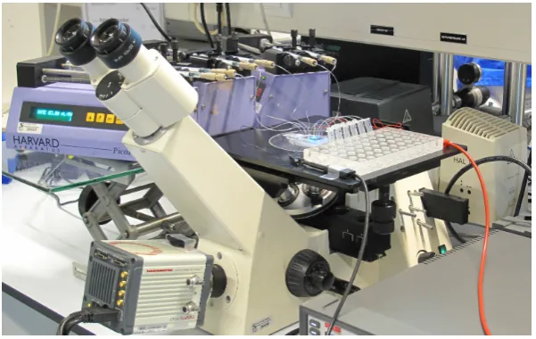
In Figure 3.2 the experimental set-up is shown. In the experiments, three microfluidic pumps with six syringes are required to pump different salt concentrated solutions through the six micro channels. The pumps are connected with six polymeric tubing to the micro chip. The end of the chip is also connected with plastic tubing, where the outflow is collected on a petri dish. The outflows are captured in separate plastic vials in order to determine the outflow concentration of each channel. To visualise the ion exchange through the hydrogels, an optical microscope is used with fluorescent dye. Furthermore, channel 1 and 6 are in the middle connected with two electrodes to the NOVA Metrohm Autolab instrument. With this instrument, different potentiostatic measurements can be performed in order to test the desalination performance with different concentrated salt solutions.

An important variable that will be changed during the experiments is the concentration of the inflow. The experiments will be performed with different concentrated sodium chloride solutions: 0.1, 1, 2, 5 and 10 mM. Another important variable that can be varied is the flow rate. For the measurements two different flow rates will be examined, namely: 3µL/min and 6µL/min. The voltage can also be varied between 0 and 10 V.

Figure 3.2: Set-up for the experiments.

Measurement procedure

Processing experimental data

In order to determine the outflow ion concentration of the channels, two different methods can be used: IV sweeps or FRA impedance measurements in combination with a fitting model. These methods will shortly be introduced in this section.

When the method of IV sweeps is used, the same order of proceedings are applicable as described in Section 3.2. In the Ohmic regime, the slope of the IV curve is equal to the resistivity, which is the reciprocal of the conductivity. When a linear calibration curve is made with known concentrations versus the conductivity, the ion concentrations of the outflow of each channel can be determined. This method is a less accurate way to determine the ion concentration, because the resistance has to be determined in the Ohmic regime. This leads to inaccuracies when verifying the slope, due to difficult observation of transition of the current regimes.

The other method that can be applied in order to determine the ion concentrations is with the use of the

FRA measurementtool in NOVA, that can be used to perform impedance spectroscopy measurements

through a frequency scan. After collecting these data, the Fit & Simulation tool in NOVA is used to determine the resistivity. An example of a fitted curve, the Nyquist plot, can be found in Figure 3.3. In this Figure -Zr ealand -Zi mag i nar yrepresent the observed real and imaginary impedances. In Figure

3.3b the used equivalent-circuit model of the electrode is given, also called the Randless circuit [13, 14]. In this Figure,Rs represents the resistance of the solution,Rc tis the charge transfer resistance,Cd l

is the double layer charging at the electrode surface and W is the Warburg Element. The Warburg Element shows the diffusion of ions in a solution. So, it contributes at low frequencies (ω→0) in the diffusionally controlled region (right side of Figure 3.3a). Ifφequals 45◦, infinite Warburg diffusion is arising. The required charge transfer resistance equals the diameter of the fitted semi-circle equals. This value (Rc t) can be determined by subtractingRsfrom the resistance of both the solution and the

resistance due to charge transfer (Rs+Rc t). These points intersect theZr ealaxis where−Zi mag i nar y

equals zero, see Figure 3.3a.

After performing these measurements, the conductivity can be verified by taking the reciprocal of the resistivity. To determine the ion concentrations of the outflow of each channel, a calibration curve has to be made. In this plot, known concentrations are plotted with their corresponding determined conductivity. This will result in a linear calibration curve.

Accuracy analysis

To show how accurate the experimental data is, an error analysis will be performed. The plotted average results of the IV sweeps will be presented with a shaded symmetric error bar in Matlab. This error bar is based on the standard deviation of the current. It is possible that the standard deviation is estimated too high, because the experiments are performed in triplicate in stead of more measurements. The same sort of accuracy analysis will be used for the determination of the ion concentration.

Model procedure

To qualitatively compare the experimental results with the theory, a numerical model is used. This model is created by the research group Soft Matter, Fluidics and Interfaces in the Multiphysics software COMSOL 5.2. The model results will be based on a flow rate of 3µL/min, 6µL/min or no flow, where fully saturation is assumed.

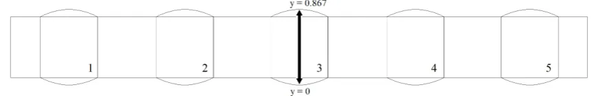
With this model a couple of outputs will be generated. Firstly, a velocity profile through the channel over a specific potential in the Ohmic regime will be made. Secondly, a graphical representation can be made of the concentration profiles over the whole channel in x-direction (see Table 3.1), based on the flow rate (0, 3 and 6µL/min). Furthermore, a concentration profile is given over the part of the channel where ion exchange will take place, the part that is enclosed by the hydrogels. Because the concentration changes over time, the time dependency will also be presented in the plot. For clarification is in Figure 3.4 the maximum width of the channel (y-direction) displayed. The position at the bottom of the component equals 0µm and at the top the maximum value of the position is 867µm. A point that should be made is that in the model, the width is made non-dimensionalised. A closer look will be taken to see if there is a difference in concentration profile if different flow rates are used (3 vs 6µL/min) and if different channel components are observed (c3 vs c5).

Figure 3.4: Numbering of channel components and the width size in y-direction.

3.3 Hypotheses

With the background information that is gathered so far, several hypotheses can be made. The hypotheses will shortly be explained in this section. These hypotheses will be tested during the experiments. The confirmation or rejection of these hypotheses will be discussed in Section 4.

When looking at Equations (3.1.1) and (3.1.2), I suppose that the efficiency parameters will not change with higher inflow ion concentrations (Ci n). When a chronopotentiometry measurement is performed

at higher concentrations of the inflow, more ions are available, so Iav g will become higher. I suppose

that the current efficiency will remain constant, because the increase of Ci nwill be levelled out with the

increased value of Iav g. Furthermore, the salt removal efficiency will also be constant over the range of

different values of Ci n. Assuming that the performance of the ion exchange through the hydrogels will

not be affected by higher concentrations and work the same as at low inflow concentrations.

Besides determining the desalination performance parameters, I will look at the IV curves at different concentrated NaCl-solutions and flow rates. At higher concentrations of the inflow, the current will be relatively higher at a certain potential. This is due to the simple fact that more ions are available to carry the current through the hydrogels. For this reason, I suppose that the slope of the IV curve is larger in the Ohmic regime when higher concentrated NaCl solutions are used.

With the difference in flow rate, I presume that a similar situation is valid. Because more ions are pumped into the channels when a higher flow rate is used, the current will be relatively higher at a certain potential. This result in a steeper IV-curve in the Ohmic regime.

In the model part, I will look at the concentration profile over the y-direction of the width of a channel component over time. First, I will look if there is a difference when no flow is used or a set flow rate of 3µL/min. I presume that the depletion zones will be larger when no flow is applied. When I look if the flow rate influences the concentration profile over time, the same expectation is made. I suppose that at higher flow rates less depletion zones are formed, due to the fact that it promotes turbulence around the hydrogel surface in the channels. In this way better mixing of ions takes places. So, at higher flow rates a relatively small edge with high concentration at the interface of the hydrogel is formed in comparison with lower flow rates. A larger part in the middle of the width of the channel component would have a similar concentration at higher flow rates, because less depletion zones are formed at higher flow rates.

4

|

Results & Discussion

In this section, the results of the experiments and model are presented together with the discussion. Besides this, the proposed hypotheses will be confirmed or rejected and an analysis of the used procedure and processing methods will be given.

4.1 Experimental results

Visualisation of formation of depletion zones

In Figure 4.1 the progression of depletion zones in the channels of the microfluidic device can be seen over time. In a period of circa 15 seconds between two frames, dark zones are created around the lower edge of each micro channel. Before the Chronopotentiometry measurement was started, the channels were fully saturated with a 0.1 mM NaCl solution containing fluorescent dye. When no air bubbles were visible in the channels, the flow rate was turned off. The full saturation of the microchannels is presented in the first image. In the consecutive images the growth of the depletion zones are visible, this is due to the applied potential of 8 V.

Figure 4.1: Formation of depletion zones in the channels due to an applied potential of 8 V without a set flow. The time span between two frames is circa 15 seconds.

In experiments with fluorescent dye, only a 0.1mM solution is used and not higher concentrated solutions. The reason is that at higher concentrations depletion zones will still be developed, but in a longer period of time. Why this occurs, will be explained later on.

Electrical characterisation of the system

0 1 2 3 4 5 6 7 8 9

Potential (V)

0 1 2 3 4 5 6 7 8 9

Current (

µ

A)

0.1 mM NaCl 1 mM NaCl 2 mM NaCl 5 mM NaCl 10 mM NaCl Concentration of inflow

Figure 4.2: Average IV sweeps with standard deviation error boxes of different inflow concentrations at a flow rate of 3µL/min.

What can be seen from Figure 4.2 is that the current increases at higher ion concentrations, which supports the hypothesis that is made. Since the charged ions facilitates the conductance of the current, the conductivity has a positively linear relation towards ion concentration. So, a larger slope in the Ohmic regime indicates a lower resistance and hence a higher conductivity. In spite of this, it is shown in the figure that in the Ohmic regime the curves lay very close to each other and the distinction is not large. A point that should be noticed is that during the measurements no off-set potential is used. This results in the fact that not all the IV-curves start at point (0,0), due to an error in the used system. At low potentials, the standard deviation error margin is also large at low potentials.

Furthermore, the distinction of the three current regimes is hardly to see in each curve, especially for the 0.1 mM NaCl-solution. Around the 1.7 V a possible transition of the Ohmic to the limiting regime can be seen for the concentrations of 2 and 5 mM. For the concentrations of 5 and 10 mM this transition is around 3 V. The limiting current (il i m) is reached when the concentration at the surface of

the membrane (Cm) becomes zero. Because at higher ion concentrations more ions are available, it will take longer before Cmreaches zero. So, when a similar potential is set at higher concentrations, the formation of depletion zones will arise slower. Hence, at a higher potential,il i mwill be reached. What

In Figure 4.3 two Chronoamperometry measurements are visible, one with an inflow concentration of 0.1 mM NaCl and the other with an inflow concentration of 5 mM NaCl. The current is measured when a potential of 2 V was applied, during a period of 700 seconds.

0 100 200 300 400 500 600 700

Time (s)

0 0.2 0.4 0.6 0.8 1 1.2 1.4 1.6

Current (

µ

A)

0.1 mM NaCl 5 mM NaCl

Concentration of inflow

Figure 4.3: Chronoamperometry measurements of two different concentrations of the inflow with an applied potential of 2 V. The connecting lines are for visualisation purposes only.

In Figure 4.4 a comparison between the two flow rates (3 & 6µL/min) is presented. The used solutions are concentrated with 0.1 mM, 1 mM and 2 mM NaCl.

0 1 2 3 4 5 6 7 8 9

Average potential (V) 0

0.5 1 1.5 2 2.5 3 3.5 4 4.5 5

Average current (

µ

A)

0.1 mM NaCl and 3µL/min 0.1 mM NaCl and 6µL/min 1 mM NaCl and 3µL/min 1 mM NaCl and 6µL/min 2 mM NaCl and 3µL/min 2 mM NaCl and 6µL/min Concentration of inflow and flow rate

Figure 4.4: Comparison of average IV sweeps for a flow rate of 3 & 6µL/min for three different inflow concentrations.

4.2 Modelling results

In this part, the modelling results are presented and discussed. All results are based on the original shaped chip. This section can be divided in two categories of results based on a set flow rate or no flow.

With flow

In Figure 4.5 two profile gradients over the whole channel are visible. These parameters are made dimensionless. Furthermore, a potential of 2 V is applied and the flow rate is set on 3µL/min. The profile gradients were made at steady state, where the time (t) equals 0.01 s. The upper part of the Figure, represents the velocity profile over the x-direction and the lower part shows the concentration gradient.

Low velocity

Low concentration

High velocity

High concentration

Figure 4.5: Normalised velocity and concentration profile with an applied potential of 2 V and a flow rate of 3µL/min (t = 0.01 s).

In the upper side of Figure 4.5 is shown that the velocity (in x-direction) in the middle of the channel is alternately high (red) and less high (orange). At the place where ion exchange take place, between the channel component and the hydrogel, the channel has a larger width. The ions are spread over a larger area when ion exchange takes place. Hence, the velocity will momentarily decrease, where it will increase again in the space between the channel components. Another visible remark for the velocity profile, is that at the ion exchange interface of the channel and the hydrogel the velocity profile gradient is blue, which indicates a very low to zero velocity. This is due to a set boundary condition, which implies that the wall of the hydrogel stands still. Due to low fluid velocities, a depletion layer is easily formed. In the lower part of Figure 4.5 the concentration profile is shown. The depletion layer at each channel component is becoming larger throughout the channel, which confirmed one of the hypothesis that is made. As can be seen in the figure, the depletion zone of c1 integrates with c2, where a larger depletion zone is visible. This integration of boundary layers increases over the whole channel.

0 0.1 0.2 0.3 0.4 0.5 0.6 0.7 0.8 0.9 Position on width channel

0 0.2 0.4 0.6 0.8 1 1.2 1.4 1.6 1.8 2 Concentration 0 0.0001 0.001 0.01 Time (in s)

Figure 4.6: Dimensionless concentration profile over y-direction of channel component 5 including time dependency (applied potential is 2 V and the flow rate is 3µL/min).

In Figure 4.6 the graphical representation of channel component 5 of Figure 4.5 is shown, with time dependency. At the start (t = 0 s), the concentration over the channel component is equally divided. It can be observed, that as function of time the depletion layer at the interface of the hydrogel increases. Hence, the depletion zone, and at the other side of the channel, the ion enriched zone increases. Over time the curve is pressed, which indicates that the middle part (with similar concentration) becomes smaller over time.

Figure 4.7 gives a comparison between location and flow rate versus the concentration profile.

0 0.1 0.2 0.3 0.4 0.5 0.6 0.7 0.8 0.9

Position on width channel 0 0.2 0.4 0.6 0.8 1 1.2 1.4 1.6 1.8 2 Concentration

c3, 3µL/min

c3, 6µL/min c5, 3µL/min

c5, 6µL/min

Channel component and flow rate

Figure 4.7: Comparison of dimensionless concentration profile over y-direction between flow rates and channel components (applied potential is 2 V and t = 0.01 s).

rates. This result supports the hypothesis that at higher flow rates the depletion zones will be smaller. Besides that, the ion enriched zones will also be smaller.

When you compare the different channel components with each other at a similar flow rate (blue and yellow or green and red) it is visible that the curves of c5 are more pressed then those of c3. This is due to more depletion formation at the last hydrogel channel, which was also shown in and explained with Figure 4.5.

Another conclusion that can be drawn from Figure 4.7 is that more depletion is formed in c3 with a flow rate of 3µL/min (blue line) than at c5 with a flow rate of 6µL/min (red line). Which indicates that the location has more influence on the desalination than the flow rate. So, when the hydrogel stacks and channels are made longer, more ion exchange could take place. Hence, a better desalination performance is reached.

No flow

In Figure 4.8 the concentration profile over the width of hc 1 over the time is given when the flow is turned off. By the reason of no flow, it does not matter for which channel component this plot is made. Moreover, a potential of 0.5 V is applied.

0 0.1 0.2 0.3 0.4 0.5 0.6 0.7 0.8 0.9

Position on width channel 0

0.2 0.4 0.6 0.8 1 1.2 1.4 1.6 1.8 2

Concentration

0

0.0001 0.001 0.003

0.005 0.007 0.01

0.03 0.05 Time (in s)

Figure 4.8: Dimensionless concentration profile over y-direction of channel component 1 including time dependency (applied potential is 0.5 V without a set flow).

4.3 Discussion of Methods & Measurements

Unfortunately, it was not possible to determine the desalination performance parameters, which was in the scope of this research. Due to measurement errors in the set-up, the current and salt removal efficiency could not be determined. The calibration curve did not gave a linear relation between the concentration and the conductivity. When using this curve, the measured concentrations of the supposed to be enriched outflows were giving desalinated values, hence ‘concentration loss’ was arisen. So, the calibration curve could not be used for the experiments due to errors in the two selected methods: FRA impedance measurements and the slope of the IV-curve.

In the case of the FRA impedance measurement, the Fit & Simulation tool gave large errors in the fitted curve in comparison with the measured data points. Thereby, the fitted curve showed a negative resistance of the solution, which cannot be valid. Regarding the second method, the conductivity was determined by the slope of the IV-curve in the Ohmic regime. From Figure 4.2 is visible that these curves are all very close to each other, even the standard deviation error boxes overlap each other. Mainly at high concentrations (5 and 10mM NaCl) the triplicate measurements were fluctuating in the Ohmic regime. Hence, both methods for determining the concentration of the outflows of the channels did not work as expected. As a consequence, the current efficiency and salt removal efficiency could not be determined with the used set-up and methods.

5

|

Conclusion

The main goal of this research was to investigate whether the hydrogels of the used microfluidic device would manage higher concentrated NaCl-solutions. This had to be researched by determining the current efficiency and the salt removal efficiency, which both are based on the concentrations of the desalinated outflows. Some difficulties occurred during the experiments, including liquid leakages, air bubble formation and difficulties in determining the outflow concentrations. Nevertheless, other measurements are performed in order to test the hypotheses. In order to justify these hypotheses, IV-and chronoamperometry measurements were performed. Besides this, an existing numerical model was used to support the theory.

From the IV-curves and the chronoamperometry plot can be noticed that the current is increased with higher concentrations and higher flow rates. More charged ions (per second) are available to carry the current through the device. Because more ions are pumped into the channels, the formation of depletion zones will take longer. Hence at higher potentials, the transition of Ohmic regime to the limiting regime takes place.

The hydrogels were not compatible enough to handle the elevated NaCl-solutions. Besides, due to the low charge density of the hydrogel, probably ion transport could not take place selectively at high concentrations. If the efficiency could have been determined, then this explanation could be validated.

From the model can be concluded that flow rate and location of the investigated channel component have influence on the formation of depletion zones. The larger the depletion zones, the more ion exchange has taken place. Higher flow rates lead to less depletion zone formation, because higher flow rates promotes turbulence and so better mixing of ions occurs near the hydrogel surface. However, when the flow rate is set too high, ion exchange would not take place in a sufficient way. Across the entire channel, larger depletion zones were formed at the end of the channel.

6

|

Recommendations

The important recommendations of this research are divided in three main categories: the measure-ment equipmeasure-ment, the adaptions of the microfluidic device and recommendations for further long-term research.

1. Measurement equipment

The used methods to determine the efficiency parameters did not work for the experiments. A calibration curve could not be made, because of the large error in the measurement equipment in order to determine the conductivity. For further research, different tools should be used to determine the concentration more accurately. For example the equipment that is used in the article of Gumuscuet al.[1]. In this article, measurements were also performed at higher potentials, which was not possible with the used equipment in this research. Besides this, the off-set potential tool should be used in the IV-curve measurements, to ensure that the curve starts at (0,0). In this way, the curves will not be shifted.

2. Adaptions of microfluidic device

Liquid leakage and air bubble formation led to difficulties during the experiments. If this could be prevented by using other chips, the experiments could better be performed. Furthermore, if hydrogels could be made from other substances in such a way that the current density and the permselectivity of the hydrogels increases, experiments at higher concentrated NaCl-solutions could better be performed. Another possibility to work at higher concentrations and higher flow rates, is to use the same micro chip with an increased length of hydrogel stacks. When the length of the hydrogel stacks in the micro chip is increased, the total exchange area and therefore also the residence time will increase. This maybe can handle the higher concentrated solutions and ensures more ion exchange, which should have a positive effect on the salt removal efficiency. In this way, no need of a larger applied potential difference is needed. This micro chip was available in the lab, although it also gave some problems. In these experiments the larger shaped micro chip had even more liquid leakage problems near the in- and outlets and at the electrode inserts. Hence, it can be concluded that a micro chip with more hydrogels could work with higher concentrated solutions, provided that a solution could be found to discourage liquid leakage and air bubble formation.

3. Long-term research

Bibliography

[1] B. Gumuscu, A. S. Haase, A. M. Benneker, M. A. Hempenius, A. van den Berg, R. G. H. Lammertink, and J. C. T. Eijkel, “Desalination by Electrodialysis Using a Stack of Patterned Ion-Selective Hydrogels on a Microfluidic Device,”Advanced Functional Materials, 2016.

[2] J. J. Krol,Monopolar and bipolar ion exchange membranes. PhD thesis, University of Twente, Enschede, August 1997.

[3] R. Kwak, G. Guan, W. K. Peng, and J. Han, “Microscale electrodialysis: Concentration profiling and vortex visualization,”Desalination, vol. 308, pp. 138–146, 2013.

[4] M. Tedesco, H. V. M. Hamelers, and P. M. Biesheuvel, “Nernst-Planck transport theory for (reverse) electrodialysis: I. Effect of co-ion transport through the membranes,”Journal of Membrane Science, vol. 510, pp. 370–381, jul 2016.

[5] Y. Tanaka, “6 - concentration polarization,” in Ion Exchange Membranes (Second Edition) (Y. Tanaka, ed.), pp. 101 – 121, Amsterdam: Elsevier, second edition ed., 2015.

[6] L. Diffusion, “IV . Transport Phenomena Lecture 16 : Concentration Polarization,”Transport, vol. 1, no. 2, pp. 1–8, 2015.

[7] P. Długołecki, B. Anet, S. J. Metz, K. Nijmeijer, and M. Wessling, “Transport limitations in ion exchange membranes at low salt concentrations,”Journal of Membrane Science, vol. 346, pp. 163– 171, jan 2010.

[8] E. I. Belova, G. Y. Lopatkova, N. D. Pismenskaya, V. V. Nikonenko, and C. Larchet, “Effect of Anion-exchange Membrane Surface Properties on Mechanisms of Overlimiting Mass Transfer,”J. Phys.

Chem., vol. 110, no. 27, pp. 13458–13469, 2006.

[9] Z. Slouka, S. Senapati, Y. Yan, and H. C. Chang, “Charge inversion, water splitting, and vortex suppression due to DNA sorption on ion-selective membranes and their ion-current signatures,”

Langmuir, vol. 29, no. 26, pp. 8275–8283, 2013.

[10] D. Hillel,Salinity Management for Sustainable Irrigation. The World Bank, aug 2000.

[11] M. Sadrzadeh and T. Mohammadi, “Treatment of sea water using electrodialysis: Current effi-ciency evaluation,”Desalination, vol. 249, pp. 279–285, nov 2009.

[12] NOVA Metrohm Autolab B.V., “NOVA Manual,” 2015.

[13] A. Lasia, “Electrochemical Impedance Spectroscopy and its Applications,” tech. rep., Département de chimie, Université de Sherbrooke Québec, 1999.

[14] C. E. Randviir, Edward P. and Banks, “Electrochemical impedance spectroscopy: an overview of bioanalytical applications,”Anal. Methods, vol. 5, no. 5, pp. 51098–1115, 2013.

A

|

Appendix - Additional figures

0 1 2 3 4 5 6 7 8 9

Potential (V)

0 0.5 1 1.5 2 2.5 3 3.5 4 4.5 5

Current (

µ

A)

0.1 mM NaCl 1 mM NaCl 2 mM NaCl Concentration of inflow

Figure A.1: Average IV sweeps of different inlet concentrations with standard deviation error box, with a flow rate of 6µL/min.

0 0.1 0.2 0.3 0.4 0.5 0.6 0.7 0.8 0.9

Position on width channel 0

0.2 0.4 0.6 0.8 1 1.2 1.4 1.6 1.8 2

Concentration

0 0.0001

0.001 0.01 Time (in s)