Negation Scope Detection for Twitter Sentiment Analysis

Negation Scope Detection for Twitter Sentiment Analysis

Johan Reitan Jørgen Faret Björn Gambäck Lars Bungum

{johan.reitan,jorgenfar}@gmail.com {gamback,larsbun}@idi.ntnu.no Department of Computer and Information Science

Norwegian University of Science and Technology Sem Sælands vei 7–9, NO–7491 Trondheim, Norway

Abstract

The paper describes the first sophisticated negation scope detection system for Twitter sentiment analysis. The system has been evaluated both on existing corpora from other domains and on a corpus of English Twitter data (tweets) annotated for nega-tion. It produces better results than what has been reported in other domains and improves the performance on tweets con-taining negation when incorporated into a state-of-the-art Twitter sentiment analyser.

1 Introduction

Exploring public opinion on various subjects has always been an important part of humans’ informa-tion gathering behaviour. Where one in the past needed to conduct surveys to learn about opinion trends, the availability of online data expressing sentiment has allowed for non-intrusive data min-ing to extract this information. Over the last decade, there has been a substantial increase in the amount of work done in the field of sentiment analysis, which has largely followed the available data, in recent years shifting the field towards Twitter data, i.e., towards Twitter sentiment analysis.

Twitter1 _{is a micro-blogging site that allows} users to write textual entries (‘tweets’) of up to 140 characters. The tweets are available through Twitter’s API and represent a real-time information stream of opinionated data. Performing language processing on tweets presents new challenges be-cause of their informal nature. Tweets often contain misspellings, slang and abbreviations, and uncon-ventional linguistic means, such as capitalization or elongation of words to show emphasis. Addition-ally, tweets contain special features likeemoticons

andhashtagsthat may have analytical value. 1_{https://www.twitter.com}

The ability to handle linguistic negation of terms is an important aspect of sentiment classification. Thevalenceof a segment of text (its communicated positive or negative attitude) can be equated to its sentimental orientation, and valence shifters are terms that change the sentimental orientation of other terms. In sentiment analysis, negators often act as valence shifters, since flipping a proposi-tion’s truth value significantly shifts, or reverses, the valence it conveys. Givón (1993) defines two forms of grammatical negation: morphological, where individual words are negated with an affix, andsyntactic, where a set of words is negated by a word or phrase; the topic of the present paper. Negators in syntactical negation, known as nega-tion cues ornegation signals, function as opera-tors, with an associated affected scope of words (Morante and Sporleder, 2012). The most common negation cue in English isnot, along with its con-tractions, such ascouldn’torisn’t(Tottie, 1991).

Negation classifiers have been developed for other domains with dramatic performance improve-ments (Section 2). However, almost all state-of-the-art Twitter sentiment analysis systems use a simple approach of marking as negated all terms from a negation cue to the next punctuation (Section 3). We present this simple model as a baseline, but im-prove on it by introducing sophisticated negation scope detection for Twitter sentiment analysis.

Several negation-annotated corpora are available, but none for the Twitter domain. To be able to evaluate Twitter negation detection and to train supervised machine learning classifiers, a corpus of tweets was annotated with negation meta-data. The new and existing corpora are detailed in Section 4.

2 Negation Scope Detection, NSD

The main application area of identifying the scope of negation, or negation scope detection (NSD), was originally biomedical texts, such as clinical reports and discharge summaries, but has in re-cent times shifted towards sentiment analysis (SA). Early solutions were typically rule-based, such as the NegFinder (Mutalik et al., 2001) and NegEx (Chapman et al., 2001) systems, that both heav-ily incorporated the use of regular expressions. NSD was the focus of a shared task at *SEM 2012 (Morante and Blanco, 2012), and in 2010 CoNLL included a similar sub-task on detecting speculation cues and their affected scope (Farkas et al., 2010). Most well-performing submissions to both tasks used supervised machine learning approaches.

Morante and Daelemans (2009) developed an NSD system that uses meta-learning for classifica-tion. They applied this approach to the CoNLL’10 shared task and achieved the best F1-score of all

participating teams. The tokens were first tagged and split into chunks, and the main algorithm then consisted of two steps: signal identification (nega-tion cue detec(nega-tion) and scope identifica(nega-tion. For the first phase, Morante and Daelemans (2009) used a decision tree to classify if a token is at the be-ginning, inside or outside a negation signal. In the second phase, a Conditional Random Fields (CRF)-based meta-learner predicted scope classes based on the output from three classifiers, a Sup-port Vector Machine (SVM), a k-nearest neighbour classifier and a CRF classifier. Zhu et al. (2010) also worked on biomedical texts and proposed a rule-based shallow semantic parsing solution: they set the negation signal as the predicate, and then use an SVM-based binary classifier to find the negated scope by identifying the correct argument(s).

Wiegand et al. (2010) surveyed the effects of NSD on SA, concluding it to be “highly relevant”. Moilanen and Pulman (2007) built an SA sys-tem with a sophisticated NSD mechanism focused on syntactic composition. Potts (2011) achieved ∼12 %better accuracy with a simple model mark-ing as negated all terms from a detected negation cue to the next punctuation. Councill et al. (2010) utilized the MaltParser (Nivre et al., 2007) for tok-enization, part-of-speech-tagging, and creation of a dependency tree to generate a feature vector for training a CRF classifier. Tested on consumer re-views, the classifier improved F1 scores by29.5 %

and11.4 %on positive resp. negative sentiments.

3 Twitter Sentiment Analysis, TSA

The typical approach to Twitter sentiment analy-sis (TSA) is a supervised machine learning system with three main steps: preprocessing, feature ex-traction, and classification. Preprocessing aims to reduce noise and consists of a variety of filters, e.g., to normalize user mentions by substituting them with the tag||T||and URLs with||U||(Agarwal et al., 2011), prefixretweets(reposts of previous content) with “RT”, and substitute letters that occur many times sequentially in elongated words (e.g.,

happyyyyyy) with one or two occurrences of the letter. It was previously common to filter out hash-tags (Selmer et al., 2013, e.g), since those when used as intended (to categorize posts by topic) offer little sentiment information; however, Mohammad (2012) shows that they add sentiment by indicating the tone of the message or the writer’s emotions.

Much recent progress in the field has been in con-nection to the International Workshop on Semantic Evaluation (SemEval), which since 2013 (Nakov et al., 2013) has included shared tasks on Sentiment Analysis in Twitter, with expression-level subtasks, to correctly classify the overall polarity of whole tweets. Many later systems have based their feature matrix on the SemEval’13 top submission (Moham-mad et al., 2013). Tang et al. (2014) define it as the state-of-the-art feature set (‘STATE’). This set will be further discussed in Section 6.1, but includes most typically used features such as word and char-actern-grams, different types of token frequencies, and a set of prior polarity sentiment lexica.

Most well-performing systems for TSA use a supervised machine learning-based classifier. An analysis of the classification algorithms used by the ten top ranking submissions to SemEval’14 (Rosenthal et al., 2014) shows that SVM and Lo-gistic Regression were the most popular choices.

Few state-of-the-art TSA systems address nega-tion systematically, but rather use the simple model described by Potts (2011), to assign a negation cue scope over all terms to the next punctuation. So do the top-3 SemEval’14 systems (Miura et al., 2014; Tang et al., 2014; Günther et al., 2014) and almost all SemEval’15 systems treating negation, includ-ing two of the top-3 (Hagen et al., 2015; Hamdan et al., 2015), although Rosenthal et al. (2015) mention negation as one area the systems focused on.

when negated tend to shift polarity and decrease their intensity, while negative terms mostly stay negative with reduced intensity. Kiritchenko et al. (2014) thus created tweet-specific sentiment lex-ica containing scores for terms in affirmative and negated contexts:NRC Hashtag Sentiment Lexicon

andSentiment140 Lexicon. The lexica added clear performance improvements (5.83 %average F1

in-crease over the five SemEval’14 data sets), even though the negated contexts were simply assumed to be from a negation cue to the next punctuation. Plotnikova et al. (2015) created one of the better SemEval’15 systems by using the heuristic of as-signing a negation cue scope over the 4 next tokens, which compares well with the 3.8 average tokens in the negation scope for our Twitter Negation Corpus (Table 1). Only one SemEval’15 system utilized an alternative treatment: Cerezo-Costas and Celix-Salgado (2015) trained a CRF-based classifier to detect the scope of what they call “denier particles” (i.e., negation) and “reversal verbs” (e.g., ‘avoid’, ‘prevent’), that reverse the polarity of the terms in their scope. The system did not perform well over all, but ranked #1 on the 2014 tweet sarcasm data. 4 Data Sets

There are negation scope corpora available for other domains and sentiment-annotated data available from the SemEval TSA tasks. However, perform-ing NSD usperform-ing supervised machine learnperform-ing re-quires a set of tweets annotated for negation cues and scopes, so such a corpus was also developed. The new and existing data sets are described below.

BioScope Corpus is a collection of bio-medical texts annotated for speculation and negation (Vincze et al., 2008). It consists of three sub-corpora: medical free texts (6,383 sentences), bio-logical full papers (2,670), and biobio-logical scientific abstracts (11,871). The free text part differs signif-icantly from the others in that it contains mainly short and concise sentences. The rate of negation, though, is even across the entire corpus:13.6 %of the sentences in the free texts,12.7 %in the full pa-pers, and13.5 %in the abstracts contain negation.

SFU Review Corpus contains 400 reviews (50 each from 8 domains such as movies and consumer products) annotated at the token level for nega-tion and speculanega-tion by Simon Fraser University (Konstantinova et al., 2012). In total, it consists of 17,263 sentences, with18.1 %containing negation.

Number of tweets 4,000 Total number of tokens 61,172 Average tokens per tweet 15.3 Average tokens per sentence 10.2 Tweets containing negation 539 Total number of scopes 615 Average cues per negated tweet 1.14 Average tokens in scope 3.8

Table 1: Twitter Negation Corpus

SemEval Twitter sentiment analysis data have been annotated using Mechanical Turk, and include training, development and test sets, as well as out-of-domain test sets. Due to Twitter’s privacy policy, the data cannot be distributed directly, but is down-loaded with a script that uses tweet IDs to match tweets with their sentiment labels. Tweets that have been deleted since the data sets’ creation are un-available, and the sets grow smaller over time. The total size of the SemEval’14 data when downloaded by us, in November 2014, was 12,754 tweets.

Twitter Negation Corpus contains 4,000 tweets downloaded through Twitter’s API and annotated by two of the authors using a web application de-veloped for this purpose. The application retrieves a tokenized tweet from the database and displays it as a container of HTML buttons, where each button represents a token. The user clicks a token to mark it as a negation cue and on corresponding tokens to mark the scope. Inter-annotator agreement was calculated at token and full scope level. The token level score is the number of tokens annotators agree on divided by the total number of tokens. It is an un-balanced measure as tokens in affirmative contexts greatly outnumber those in negated. Full scope agreement entails that annotator scopes match com-pletely. Token level agreement was98.9 %and full scope agreement73.8 %. All scope conflicts were reviewed and resolved after discussion.

aint cannot cant darent didnt doesnt dont hadnt hardly hasnt havent havnt isnt lack lacking lacks neither never no nobody

none nor not nothing nowhere

mightnt mustnt neednt oughtnt shant

shouldnt wasnt without wouldnt *n’t Table 2: Lexicon of negation cues

5 Negation Scope Detection Experiments Two classifiers were created: one to detect the scope of negation and one to assign sentiment. The negation classifier was used in the feature extrac-tion process for the sentiment classifier (Secextrac-tion 6). Negation scope detection (NSD) is a binary clas-sification problem, where each token is determined to be either in an affirmative or a negated context. For NSD experiments, we report precision (P), re-call (R), F1score, and thepercentage of correctly classified scopes (PCS): For classification tasks where the output is a sequence, metrics that only consider individual units regardless of their order are often insufficient. PCS measures the accuracy of a scope classifier: a scope is considered correctly classified if, for a given negation cue, every token in its associated scope has been correctly marked.

5.1 Negation Classifier Architecture

The classification algorithm consists of two steps: negation cue detection and scope identification. Cue detection is performed by a pattern-matching approach with a lexicon of explicit cues adopted from Councill et al. (2010), as shown in Table 2, where*n’tmatches all strings with the suffixn’t. Note that this list is more extensive than the one of Potts (2011), used in many SemEval systems. Four cues on Potts’ list are not in Table 2 (noone, couldnt, wont, arent), while the 17 cues in italics are not listed by Potts. An inspection of the 37 cues appearing in the Twitter Negation Corpus revealed seven more cues / spelling variants included on nei-ther list (idk, dnt, cudnt, ain, eint, neva, neeeever). Tweets are preprocessed with the TweeboParser dependency parser (Kong et al., 2014), that per-forms tokenisation, part-of-speech tagging and parsing, labeling each token with its dependency head. A dependency-based binary CRF classifier then for each token determines whether it is in a negated or affirmative context. The CRF implemen-tation by Okazaki (2007) is used, with a Python binding created by Peng and Korobov (2014).

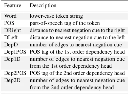
Feature Description

Word lower-case token string POS part-of-speech tag of the token

DRight distance to nearest negation cue to the right DLeft distance to nearest negation cue to the left DepD number of edges to nearest negation cue Dep1POS POS tag of the 1st order dependency head Dep1D number of edges to nearest negation cue

from the 1st order dependency head Dep2POS POS tag of the 2nd order dependency head Dep2D number of edges to nearest negation cue

from the 2nd order dependency head Table 3: Negation classifier feature set

The classifier is a Twitter-tailored version of the system described by Councill et al. (2010) with one change: the dependency distance from each token to the closest negation cue has been added to the feature set, which is shown in Table 3. The distances (DRight and DLeft) are the minimun lin-ear token-wise distances, i.e., the number of tokens from one token to another. Dependency distance (DepD) is calculated as the minimum number of edges that must be traversed in a dependency tree to move from one token, to another. The classifier takes a parameter,max distance, that specifies the maximum distance to be considered (all longer dis-tances are treated as being equivalent). This applies to both linear distance and dependency distance.

5.2 Negation Cue Detection

The created Conditional Random Fields negation classifier was evaluated on the Twitter Negation Corpus. The data set was split into two subsets: a development set and an evaluation set. The develop-ment set consists of 3,000 tweets and the evaluation set of 1,000 tweets. To ensure more reliable train-ing and testtrain-ing, given the heavy label imbalance of the corpus, the split was stratified, with the same ratio of tweets containing negation in both subsets.

The actual negation cues in the annotated train-ing data are used when traintrain-ing the classifier, but a lexicon-based cue detection approach is taken during classification. When applied to the Twitter Negation Corpus, the cue detector achieved a pre-cision of 0.873 with a recall of 0.976, and hence an F1 score of 0.922. In comparison, Morante

Data NSD model P R F1 PCS

Test

Sophisticated 0.972 0.923 0.853 64.5 Gold standard 0.841 0.956 0.895 66.3 Simple 0.591 0.962 0.733 43.1 Train Sophisticated 0.849 0.891 0.868 66.3

Table 4: Negation classifier performance

Inspection of the cue detection output reveals that the classifier mainly struggles with the sepa-ration of words used both as negators and excla-mations. By far the most significant of these isno, with 35 of its 90 occurrences in the corpus being as a non-cue; often it occurs as a determiner function-ing as a negator (e.g., “there were no letters this morning”), but it may occur as an exclamation (e.g., “No, I’m not ready yet” and “No! Don’t touch it”). Despite the high recall, cue outliers such as

dnt neva, or cudnt could potentially be detected by using word-clusters. We expanded the lexi-con of negation cues to lexi-contain the whole set of Tweet NLP word clusters created by Owoputi et al. (2013) for each lexical item. Recall was slightly increased, to 0.992, but precision suffered a dra-matic decrease to 0.535, since the clusters are too inclusive. More finely-grained word clusters could possibly increase recall without hurting precision.

5.3 NSD Classifier Performance

To determine the optimal parameter values, a 7-fold stratified cross validation grid search was per-formed on the development set over the L1 and L2 CRF penalty coefficients, C1 andC2 with a parameter space of{10−4_,10−3_,10−2_,0.1,1,10},

in addition tomax distance(see Section 5.1) with a[5,10]parameter space. The identified optimal setting wasC1=0.1, C2=1,max distance=7.

The performance of thesophisticatednegation scope classifier with the parameter set selected through grid search was evaluated on the held-out test data. The classifier was also tested on the same evaluation set with gold standard cue detection (i.e., with perfect negation signal identification).

To establish a baseline for negation scope detec-tion on the Twitter Negadetec-tion Corpus, we also im-plemented the simple model described in Section 2 and used by almost all SemEval TSA systems han-dling negation: When a negation cue is detected, all terms from the cue to the next punctuation are considered negated. Note though, that by using an extended cue dictionary, oursimplebaseline poten-tially slightly improves on state-of-the-art models.

Data Classifier P R F1 PCS

SFU Sophisticated 0.668 0.874 0.757 43.5

BioScope

full CRF_MetaLearn 0.808 0.708 0.755 53.7_{0.722 0.697 0.709 41.0} Sophisticated 0.660 0.610 0.634 42.6 Simple 0.583 0.688 0.631 43.7 SSP 0.582 0.563 0.572 64.0 Table 5: Out-of-domain NSD performance

Results from the test run on the evaluation data, and the test on the evaluation set with gold stan-dard cue detection are shown in Table 4, together with the simple baseline, as well as a 7-fold cross validation on the development set.

The classifier achieves very good results. The run on the evaluation set produces an F1 score of

0.853, which is considerably higher than the base-line. It also outperforms Councill et al. (2010) who achieved an F1 score of 0.800 when applying a

similar system to their customer review corpus.

5.4 Out-of-Domain Performance

Although the negation classifier is a Twitter-tailored implementation of the system described by Councill et al. (2010) with minor modifications the use of a different CRF implementation, POS-tagger and dependency parser may lead to consid-erable performance differences. To explore the out-of-domain capacity of the classifier, it was eval-uated on the SFU Review corpus and the biological full paper part of BioScope, as that sub-corpus has proved to be difficult for negation identification.

Table 5 shows the 5-fold cross-validated perfor-mance of the sophisticated negation scope identifier on both corpora, as well as the simple baseline on Bioscope together with the results reported on the same data for the approaches described in Section 2. ‘CRF’ denotes the CRF-based system from Coun-cill et al. (2010), ‘MetaLearn’ the meta-learner of Morante and Daelemans (2009), and ‘SSP’ the shal-low semantic parsing solution by Zhu et al. (2010). As can be seen, the twitter-trained sophisticated negation classifier performs reasonably well on the SFU Review Corpus, but struggles when applied to BioScope, as expected. It is outperformed in terms of F1score by Councill et al. (2010) and Morante

and Daelemans (2009), but reaches a slightly better PCS than the latter system. The modest F1 score

Notably, the simple model is a strong baseline, which actually outperforms the shallow parser on F1 score and the meta-learner on percentage of

correctly classified scopes (PCS).

6 An NSD-enhanced Sentiment Classifier The Twitter sentiment analysis includes three steps: preprocessing, feature extraction, and either train-ing the classifier or classifytrain-ing samples. A Support Vector Machine classifier is used as it is a state-of-the-art learning algorithm proven effective on text categorization tasks, and robust on large feature spaces. We employ the SVM implementationSVC from Scikit-learn (Pedregosa et al., 2011), which is based on libsvm (Chang and Lin, 2011).

6.1 Sentiment Classifier Architecture

The preprocessing step substitutes newline and tab characters with spaces, user mentions with the string “@someuser”, and URLs with “http://someurl” using a slightly modified

regu-lar expression by@stephenhay,2_{matching URLs} starting with protocol specifiers or only “www”.

The feature extraction step elicitates characteris-tics based on the STATE set, as shown in Table 6; the top four features are affected by linguistic nega-tion, the rest are not. There are two term frequency-inverse document frequency (TF-IDF) vectorizers, for wordn-grams (1≤n≤4) and forcharacter

n-grams(3≤n≤5). Both ignore common English stop words, convert all characters to lower case, and select the 1,000 features with highest TF-IDF scores. Tokens in a negation scope are appended the string_NEG. Thenegated tokensfeature is sim-ply a count of the tokens in a negated context.

TheNRC Hashtag Sentiment Lexiconand Sen-timent140 Lexicon(Kiritchenko et al., 2014) con-tain sentiment scores for words in negated contexts. For lookups, the first negated word in a negation scope is appended with_NEGFIRST, and the rest with_NEG. The sentiment lexica feature vectors are adopted from Kiritchenko et al. (2014) and con-tain the number of tokens withscore(w)6= 0, the total score, the maximal score, and the score of the last token in the tweet. We also useThe MPQA Sub-jectivity Lexicon(Wilson et al., 2005),Bing Liu’s Opinion Lexicon(Ding et al., 2008), and theNRC Emotion Lexicon(Mohammad and Turney, 2010), assigning scores of+/−2 for strong and +/−1 for weak degrees of sentiment. The resulting four

2_{mathiasbynens.be/demo/url-regex}

Feature Description

Wordn-grams contiguous token sequences Charn-grams contiguous character sequences Negated tokens number of negated tokens Sentiment lexica feature set for each lexicon Clusters tokens from ‘1000 word clusters’ POS part-of-speech tag frequency All caps upper-case tokens

Elongated tokens with repeated characters Emoticons positive and negative emoticons Punctuation punctuation mark sequences Hashtags number of hashtags

Table 6: Sentiment classifier STATE feature set

feature vectors contain the sum of positive and neg-ative scores for tokens in affirmneg-ative and negated contexts, equivalently to Kiritchenko et al. (2014). Instead of adding only the presence of words from each of the 1000 clusters from CMU’s Tweet NLP tool3 _{in theclustersfeature, as Kiritchenko} et al. (2014) did, we count occurrences for each cluster and represent them with a feature. Input to thePOSfeature is obtained from the Twitter part-of-speech tagger (Owoputi et al., 2013). The emoti-consfeature is the number of happy and sad emoti-cons, and whether a tweet’s last token is happy or a sad. Theall-caps,elongated(tokens with char-acters repeated more than two times),punctuation

(exclamation or question marks), andhashtag fea-tures are straight-forward counts of the number of tokens of each type. All the matrices from the different parts of the feature extraction are concate-nated column-wise into the final feature matrix, and scaled in order to be suitable as input to a classifier.

The classifier step declares which classifier to use, along with its default parameters. It is passed the resulting feature matrix from the feature ex-traction, with which it creates the decision space if training, or classifies samples if predicting. Us-ing the negation scope classifier with the param-eters identified in Section 5.3, a grid search was performed over the entire Twitter2013-train data set using stratified 10-fold cross validation to find theCandγ parameters for the SVM classifier. A preliminary coarse search showed the radial ba-sis function (RBF) kernel to yield the best results, although most state-of-the-art sentiment classifica-tion systems use a linear kernel.

A finer parameter space was then examined. The surface plots in Figure 1 display the effects of theC

10−7₁₀−6₁₀−5₁₀−4 0.2

0.4 0.6

γ

F1

10

−

7

10

−

6

10

−

5

10

−

4

0

.

2

0

.

4

0

.

6

γ

F

1

10 20

0.2 0.4 0.6

C

F1

10

20

0

.

2

0

.

4

0

.

6

C

F

1

Figure 1: SVM grid search F1scores forγ andC

andγparameters on the classifier’s F1 score. The

combination of parameters that scored best was

C = 10andγ ≈ 5.6∗10−6_{, marked by circles.}

IncreasingCbeyond10gives no notable change in F1score. The combination of a smallγ and higher

values ofCmeans that the classifier is quite gener-alized, and that increasingC(regularizing further) makes no difference. It also suggests that the data is noisy, requiring a great deal of generalization.

In order to allow a user to query Twitter for a search phrase on live data, the classifier is wrapped in a web application using the Django web frame-work.4 _{The resulting tweet hits are classified using} a pre-trained classifier, and presented to the user indicating their sentiment polarities. The total dis-tribution of polarity is also displayed as a graph to give the user an impression of the overall opinion.

6.2 Sentiment Classifier Performance

The SVM was trained on the Twitter2013-train set using the parameters identified through grid search, and tested on the Twitter2014-test and Twitter2013-test sets, scoring as in Table 7. Sentiment classi-fication is here treated as a three-class task, with the labels positive, negative, and objective/neutral. In addition to precision, recall, and F1 for each

class, we report themacro-averageof each met-ric across all classes. Macro-averaging disregards class imbalance and is calculated by taking the av-erage of the classification metric outputs for each label, equally weighting each label, regardless of its number of samples. The last column of the table shows thesupport: the number of samples for each label in the test set.

As can be seen in the table, the classifier per-formed worst on negative samples. Figure 2 dis-plays the confusion matrices for the Twitter2013-test set (the Twitter2014 matrices look similar). If there were perfect correlation between true and pre-dicted labels, the diagonals would be completely red. However, the confusion matrices show (clearer in the normalized version) that the classifier is quite biased towards the neutral label (illustrated with ),

4_{https://djangoproject.com}

Label P R F1 Support

Twitter2014-test

positive 0.863 0.589 0.700 805 neutral 0.568 0.872 0.688 572 negative 0.717 0.487 0.580 156 avg / total 0.738 0.684 0.684 1533

Twitter2013-test

positive 0.851 0.581 0.691 1273 neutral 0.627 0.898 0.739 1369 negative 0.711 0.426 0.533 467 avg / total 0.731 0.697 0.688 3109

Table 7: Sentiment classifier performance

Predicted label

True

label

Without normalization

0 500 1,000

Predicted label

With normalization

0.2 0.4 0.6 0.8 1

Figure 2: Sentiment classifier confusion matrices

as can be seen from the warm colours in the and true label cells of the predicted label column, in particular misclassifying negative samples. This is likely an effect of the imbalanced training set, where neutral samples greatly outnumber negative.

6.3 TSA Feature Ablation Study

The results of an ablation study of the TSA clas-sifier are shown in Table 8, where the all rows (n-grams/counts) refer to removing all features in that group. Most apparently, thesentiment lexica

feature has the greatest impact on classifier per-formance, especially on the Twitter2013-test set. This may be since the most important lexica (Senti-ment140 and NRC Hashtag Sentiment) were cre-ated at the same time as the Twitter2013 data, and could be more accurate on the language used then.

Thecharactern-gramfeature slightly damages performance on the Twitter2014-test set, although making a positive contribution on the Twitter2013 data. This is most likely caused by noise in the data, but the feature could be sensitive to certain details that appeared after the Twitter2013 data collection.

The majority of the count features do not impose considerable changes in performance, although the

Features ₂₀₁₄Twitter test₂₀₁₃

All 0.684 0.688

n-grams

−wordn-grams 0.672 0.674 −charn-grams 0.688 0.676 −alln-grams 0.664 0.667 −sentiment lexica 0.665 0.657

frequenc

y

count

features

−clusters 0.666 0.677 −POS 0.684 0.685 −all caps 0.685 0.689 −elongated 0.682 0.687 −emoticons 0.681 0.688 −punctuation 0.682 0.688 −hashtag 0.684 0.688 −negation 0.684 0.688 −all counts 0.665 0.671 Table 8: Sentiment classifier ablation (F1scores)

However, the Tweet NLP clusters feature has a large impact, as anticipated. Tweets contain many misspellings and unusual abbreviations and expres-sions, and the purpose of this feature is to make generalizations by counting the occurrences of clus-ters that include similar words.

6.4 Effect of Negation Scope Detection

Table 9 shows the effects of performing negation scope detection on several variations of the sen-timent classification system and data sets. The first six rows give results from experiments using the Twitter2013-training and Twitter2014-test sets, and the remaining rows results when using only a subset of the data: tweets that contain negation, as determined by our NSD system. The rows are grouped into four segments, where each segment shows scores for a classifier using either no, simple or sophisticated negation scope detection. The seg-ments represent different feature sets, either using

allfeatures or only the features that are directly affected bynegation: word and charactern-grams, sentiment lexica, and negation counts.

In every case, taking negation into account us-ing either the simple or the sophisticated method improves the F1score considerably. Using all the

data, the sophisticated solution scores marginally better than the simple one, but it improves more clearly upon the simple method on the negated part of the data, with F1 improvements ranging from 4.5 %to6.1 %(i.e., from 0.029 to 0.039 F1score).

Features NSD method P R F1

All tweets (training and test sets)

all

No 0.730 0.659 0.653

Simple 0.738 0.676 0.675

Sophisticated 0.738 0.684 0.684

ne

gation

No 0.705 0.618 0.601

Simple 0.728 0.663 0.662

Sophisticated 0.729 0.667 0.665 Only tweets containing negation

all

No 0.598 0.599 0.585

Simple 0.653 0.654 0.644

Sophisticated 0.675 0.682 0.673

ne

gation

No 0.609 0.604 0.586

Simple 0.648 0.654 0.633

Sophisticated 0.681 0.696 0.672

Table 9: Sentiment classification results

7 Conclusion and Future Work

The paper has introduced a sophisticated approach to negation scope detection (NSD) for Twitter sen-timent analysis. The system consists of two parts: a negation cue detector and a negation scope clas-sifier. The cue detector uses a lexicon lookup that yields high recall, but modest precision. However, the negation scope classifier still produces better results than observed in other domains: an F1score

of0.853with64.5 %correctly classified scopes, in-dicating that the Conditional Random Fields-based scope classifier is able to identify the trend of cer-tain dictionary cues being misclassified.

A sentiment classifier for Twitter data was also developed, incorporating several features that ben-efit from negation scope detection. The results confirm that taking negation into account in gen-eral improves sentiment classification performance significantly, and that using a sophisticated NSD system slightly improves the performance further. The negation cue variation in the Twitter data was quite low, but due to part-of-speech ambiguity it was for some tokens unclear whether or not they functioned as a negation signal. A more intricate cue detector could in the future aim to resolve this.

References

Apoorv Agarwal, Boyi Xie, Ilia Vovsha, Owen Rambow, and Rebecca Passonneau. 2011. Sentiment analysis of Twitter data. InProceedings of the 49th Annual Meeting of the Association for Computational Linguistics: Human Lan-guage Technologies, pages 30–38, Portland, Oregon, June. ACL. Workshop on Languages in Social Media.

Héctor Cerezo-Costas and Diego Celix-Salgado. 2015. Gradiant-analytics: Training polarity shifters with CRFs for message level polarity detection. InProceedings of the 9th International Workshop on Semantic Evaluation, pages 539–544, Denver, Colorado, June. ACL.

Chih-Chung Chang and Chih-Jen Lin. 2011. LIBSVM: A library for support vector machines. ACM Transactions on Intelligent Systems and Technology, 2(3):27:1–27:27, April.

Wendy W. Chapman, Will Bridewell, Paul Hanbury, Gregory F. Cooper, and Bruce G. Buchanan. 2001. A simple al-gorithm for identifying negated findings and diseases in discharge summaries. Journal of Biomedical Informatics, 34(5):301–310, October.

Isaac G. Councill, Ryan McDonald, and Leonid Velikovich. 2010. What’s great and what’s not: learning to classify the scope of negation for improved sentiment analysis. In

Proceedings of the 48th Annual Meeting of the Association for Computational Linguistics, pages 51–59, Uppsala, Swe-den, July. ACL. Workshop on Negation and Speculation in Natural Language Processing.

Xiaowen Ding, Bing Liu, and Philip S. Yu. 2008. A holistic lexicon-based approach to opinion mining. In Proceed-ings of the 2008 International Conference on Web Search and Data Mining, pages 231–240, Stanford, California, February. ACM.

Richárd Farkas, Veronika Vincze, György Móra, János Csirik, and György Szarvas. 2010. The CoNLL-2010 shared task: Learning to detect hedges and their scope in natural language text. InProceedings of the 14th Conference on Computational Natural Language Learning, pages 1–12, Uppsala, Sweden, July. ACL.

Talmy Givón. 1993. English grammar: A function-based introduction. John Benjamins, Amsterdam, The Nether-lands.

Tobias Günther, Jean Vancoppenolle, and Richard Johansson. 2014. RTRGO: Enhancing the GU-MLT-LT system for sentiment analysis of short messages. InProceedings of the 8th International Workshop on Semantic Evaluation, pages 497–502, Dublin, Ireland, August. ACL.

Matthias Hagen, Martin Potthast, Michael Büchner, and Benno Stein. 2015. Webis: An ensemble for Twitter sen-timent detection. InProceedings of the 9th International Workshop on Semantic Evaluation, pages 582–589, Denver, Colorado, June. ACL.

Hussam Hamdan, Patrice Bellot, and Frederic Bechet. 2015. Lsislif: Feature extraction and label weighting for senti-ment analysis in Twitter. InProceedings of the 9th Interna-tional Workshop on Semantic Evaluation, pages 568–573, Denver, Colorado, June. ACL.

Svetlana Kiritchenko, Xiaodan Zhu, and Saif M. Mohammad. 2014. Sentiment analysis of short informal texts. Journal of Artificial Intelligence Research, 50:723–762, August.

Lingpeng Kong, Nathan Schneider, Swabha Swayamdipta, Archna Bhatia, Chris Dyer, and Noah A. Smith. 2014. A dependency parser for tweets. InProceedings of the 2014 Conference on Empirical Methods in Natural Language Processing, pages 1001–1012, Doha, Qatar, October. ACL. Natalia Konstantinova, Sheila C.M. de Sousa, Noa P. Cruz, Manuel J. Maña, Maite Taboada, and Ruslan Mitkov. 2012. A review corpus annotated for negation, speculation and their scope. InProceedings of the 8th International Con-ference on Language Resources and Evaluation, pages 3190–3195, Istanbul, Turkey, May. ELRA.

Yasuhide Miura, Shigeyuki Sakaki, Keigo Hattori, and Tomoko Ohkuma. 2014. TeamX: A sentiment analyzer with enhanced lexicon mapping and weighting scheme for unbalanced data. InProceedings of the 8th International Workshop on Semantic Evaluation, pages 628–632, Dublin, Ireland, August. ACL.

Saif Mohammad and Peter Turney. 2010. Emotions evoked by common words and phrases: Using Mechanical Turk to create an emotion lexicon. InProceedings of the 2010 Human Language Technology Conference of the North American Chapter of the Association for Computational Linguistics, pages 26–34, Los Angeles, California, June. ACL. Workshop on Computational Approaches to Analy-sis and Generation of Emotion in Text.

Saif Mohammad, Svetlana Kiritchenko, and Xiaodan Zhu. 2013. NRC-Canada: Building the state-of-the-art in sen-timent analysis of tweets. InSecond Joint Conference on Lexical and Computational Semantics (*SEM), Volume 2: Proceedings of the 7th International Workshop on Semantic Evaluation, SemEval ’13, pages 321–327, Atlanta, Georgia, June. ACL.

Saif Mohammad. 2012. #Emotional tweets. In First Joint Conference on Lexical and Computational Semantics (*SEM), Volume 2: Proceedings of the 6th International Workshop on Semantic Evaluation, pages 246–255, Mon-tréal, Canada, June. ACL.

Karo Moilanen and Stephen Pulman. 2007. Sentiment com-position. InProceedings of the 6th International Confer-ence on Recent Advances in Natural Language Processing, pages 378–382, Borovets, Bulgaria, September.

Roser Morante and Eduardo Blanco. 2012. * SEM 2012 shared task: Resolving the scope and focus of negation. In

First Joint Conference on Lexical and Computational Se-mantics (*SEM), Volume 2: Proceedings of the 6th Interna-tional Workshop on Semantic Evaluation, pages 265–274, Montréal, Canada, June. ACL.

Roser Morante and Walter Daelemans. 2009. A metalearning approach to processing the scope of negation. In Proceed-ings of the 13th Conference on Computational Natural Language Learning, pages 21–29, Boulder, Colorado, June. ACL.

Roser Morante and Caroline Sporleder. 2012. Modality and negation: An introduction to the special issue. Computa-tional Linguistics, 38(2):223–260.

Preslav Nakov, Zornitsa Kozareva, Sara Rosenthal, Veselin Stoyanov, Alan Ritter, and Theresa Wilson. 2013. SemEval-2013 Task 2: Sentiment analysis in Twitter. In

Second Joint Conference on Lexical and Computational Semantics (*SEM), Volume 2: Proceedings of the 7th Inter-national Workshop on Semantic Evaluation, SemEval ’13, pages 312–320, Atlanta, Georgia, June. ACL.

Joakim Nivre, Johan Hall, Jens Nilsson, Atanas Chanev, Gül¸sen Eryi˘git, Sandra Kübler, Svetoslav Marinov, and Erwin Marsi. 2007. MaltParser: A language-independent system for data-driven dependency parsing.Natural Lan-guage Engineering, 13(2):95–135, January.

Naoaki Okazaki. 2007. CRFsuite: a fast implementation of conditional random fields (CRFs).

www.chokkan.org/software/crfsuite/. Olutobi Owoputi, Brendan O’Connor, Chris Dyer, Kevin

Gim-pel, Nathan Schneider, and Noah A. Smith. 2013. Im-proved part-of-speech tagging for online conversational text with word clusters. InProceedings of the 2013 Confer-ence of the North American Chapter of the Association for Computational Linguistics: Human Language Technolo-gies, pages 380–390, Atlanta, Georgia, June. ACL. Fabian Pedregosa, Gaël Varoquaux, Alexandre Gramfort,

Vin-cent Michel, Bertrand Thirion, Olivier Grisel, Mathieu Blondel, Peter Prettenhofer, Ron Weiss, Vincent Dubourg, Jake Vanderplas, Alexandre Passos, David Cournapeau, Matthieu Brucher, Matthieu Perrot, and Édouard Duch-esnay. 2011. Scikit-learn: Machine learning in Python.

Journal of Machine Learning Research, 12(1):2825–2830. Terry Peng and Mikhail Korobov. 2014. python-crfsuite.

github.com/tpeng/python-crfsuite.

Nataliia Plotnikova, Micha Kohl, Kevin Volkert, Stefan Evert, Andreas Lerner, Natalie Dykes, and Heiko Ermer. 2015. KLUEless: Polarity classification and association. In Pro-ceedings of the 9th International Workshop on Semantic Evaluation, pages 619–625, Denver, Colorado, June. ACL. Christopher Potts. 2011. Sentiment symposium tutorial. In

Sentiment Analysis Symposium, San Francisco, California, November. Alta Plana Corporation.

http://sentiment.christopherpotts.net/. Sara Rosenthal, Alan Ritter, Preslav Nakov, and Veselin

Stoy-anov. 2014. SemEval-2014 Task 9: Sentiment analysis in Twitter. InProceedings of the 8th International Workshop on Semantic Evaluation, pages 73–80, Dublin, Ireland, August. ACL.

Sara Rosenthal, Preslav Nakov, Svetlana Kiritchenko, Saif Mohammad, Alan Ritter, and Veselin Stoyanov. 2015. SemEval-2015 Task 10: Sentiment analysis in Twitter. In

Proceedings of the 9th International Workshop on Semantic Evaluation, pages 451–463, Denver, Colorado, June. ACL. Øyvind Selmer, Mikael Brevik, Björn Gambäck, and Lars Bungum. 2013. NTNU: Domain semi-independent short message sentiment classification. InSecond Joint Con-ference on Lexical and Computational Semantics (*SEM), Volume 2: Proceedings of the 7th International Workshop on Semantic Evaluation, SemEval ’13, pages 430–437, Atlanta, Georgia, June. ACL.

Duyu Tang, Furu Wei, Bing Qin, Ting Liu, and Ming Zhou. 2014. Coooolll: A deep learning system for Twitter senti-ment classification. InProceedings of the 8th International Workshop on Semantic Evaluation, pages 208–212, Dublin, Ireland, August. ACL.

Gunnel Tottie. 1991.Negation in English Speech and Writ-ing: A Study in Variation. Academic Press, San Diego, California.

Veronika Vincze, György Szarvas, Richárd Farkas, György Móra, and János Csirik. 2008. The BioScope corpus: biomedical texts annotated for uncertainty, negation and their scopes.BMC Bioinformatics, 9(Suppl 11):S9, Novem-ber.

Michael Wiegand, Alexandra Balahur, Benjamin Roth, Diet-rich Klakow, and Andrés Montoyo. 2010. A survey on the role of negation in sentiment analysis. InProceedings of the 48th Annual Meeting of the Association for Compu-tational Linguistics, pages 60–68, Uppsala, Sweden, July. ACL. Workshop on Negation and Speculation in Natural Language Processing.

Theresa Wilson, Paul Hoffmann, Swapna Somasundaran, Ja-son Kessler, Janyce Wiebe, Yejin Choi, Claire Cardie, Ellen Riloff, and Siddharth Patwardhan. 2005. OpinionFinder: A system for subjectivity analysis. InProceedings of the 2005 Human Language Technology Conference and Conference on Empirical Methods in Natural Language Processing, pages 34–35, Vancouver, British Columbia, Canada, October. ACL. Demonstration Abstracts. Qiaoming Zhu, Junhui Li, Hongling Wang, and Guodong