Estimating and visualizing language similarities using weighted alignment and force directed graph layout

Estimating and visualizing language similarities using weighted

alignment and force-directed graph layout

Gerhard J¨ager

University of T¨ubingen, Department of Linguistics [email protected]

Abstract

The paper reports several studies about quantifying language similarity via pho-netic alignment of core vocabulary items (taken from Wichman’s Automated Simi-larity Judgement Program data base). It turns out that weighted alignment accord-ing to the Needleman-Wunsch algorithm yields best results.

For visualization and data exploration pur-poses, we used an implementation of the Fruchterman-Reingold algorithm, a version of force directed graph layout. This soft-ware projects large amounts of data points to a two- or three-dimensional structure in such a way that groups of mutually similar items form spatial clusters.

The exploratory studies conducted along these ways lead to suggestive results that provide evidence for historical relation-ships beyond the traditionally recognized language families.

1 Introduction

The Automated Similarity Judgment Program (Wichmann et al., 2010) is a collection of 40-item Swadesh lists from more than 5,000 languages. The vocabulary items are all given in a uniform, if coarse-grained, phonetic transcription.

In this project, we explore various ways to com-pute the pairwise similarities of these languages based on sequence alignment of translation pairs. As the 40 concepts that are covered in the data base are usually thought to be resistant against borrowing, these similarities provide information about genetic relationships between languages.

To visualize and explore the emerging pat-terns, we make use ofForce Directed Graph

Lay-out. More specifically, we use the CLANS1 im-plementation of the Fruchterman-Reingold algo-rithm (Frickey and Lupas, 2004). This algoalgo-rithm takes a similarity matrix as input. Each data point is treated as a physical particle. There is a re-pelling force between any two particles — you may think of the particles as electrically charged with the same polarity. Similarities are treated as attracting forces, with a strength that is positively related to the similarity between the correspond-ing data points.

All data points are arranged in a two- or three-dimensional space. The algorithm simulates the movement of the particles along the resulting force vector and will eventually converge towards an energy minimum.

In the final state, groups of mutually similar data items form spatial clusters, and the distance between such clusters provides information about their cumulative similarity.

This approach has proven useful in bioinfor-matics, for instance to study the evolutionary his-tory of protein sequences. Unlike more com-monly used methods like SplitsTree (or other phy-logenetic tree algorithms), CLANS does not as-sume an underlying tree structure; neither does it compute a hypothetical phylogenetic tree or net-work. The authors of this software package, Tan-cred Frickey and Andrei Lupas, argue that this approach is advantageous especially in situations were a large amount of low-quality data are avail-able:

“An alternative approach [...] is the visualization of all-against-all pairwise

1_{ClusterANalysis ofSequences; freely available from}

similarities. This method can han-dle unrefined, unaligned data, includ-ing non-homologous sequences. Un-like phylogenetic reconstruction it be-comes more accurate with an increas-ing number of sequences, as the larger number of pairwise relationships aver-age out the spurious matches that are the crux of simpler pairwise similarity-based analyses.” (Frickey and Lupas 2004, 3702)

This paper investigates two issues, that are re-lated to the two topics of the workshop respec-tively:

• Which similarity measures over language pairs based on the ASJP data are apt to sup-ply information about genetic relationships between languages?

• What are the advantages and disadvantages of a visualization method such as CLANS, as compared to the more commonly used phy-logenetic tree algorithms, when applied to large scale language comparison?

2 Comparing similarity measures

2.1 The LDND distance measure

In Bakker et al. (2009) a distance measure is de-fined that is based on the Levenshtein distance (= edit distance) between words from the two lan-guages to be compared. Suppose two lanlan-guages, L1 andL2, are to be compared. In a first step, the normalized Levenshtein distancesbetween all word pairs from L1andL2 are computed. (Ide-ally this should be 40 word pairs, but some data are missing in the data base.) This measure is de-fined as

nld(x, y)=. dLev(x, y)

max(l(x), l(y)). (1)

The normalization term ensures that word length does not affect the distance measure.

IfL1andL2have small sound inventories with a large overlap (which is frequently the case for tonal languages), the distances between words from L1 and L2 will be low for non-cognates because of the high probability of chance simi-larities. If L1 and L2 have large sound inven-tories with little overlap, the distance between

Figure 1: Simple alignment

non-cognates will be low in comparison. To cor-rect for this effect, Bakker et al. (2009) normal-ize the distance between two synonymous words fromL1andL2by defining the normalized Lev-enshtein distance by the average distance between all words fromL1 andL2 that are non synony-mous (39×40 = 1,560pairs if no data are miss-ing). TheNDLDdistance betweenL1andL2is defined as the average doubly normalized Leven-shtein distance between synonymous word pairs fromL1and L2. (LDND is a distance measure rather than a similarity measure, but it is straight-forward to transform the one type of measure into the other.)

In the remainder of this section, I will propose an improvement of LDND in two aspects:

• using weighted sequence alignment based on phonetic similarity, and

• correcting for the variance of alignments us-ing an information theoretic distance mea-sure.

2.2 Weighted alignment

There is a parallel here to problems in bioin-formatics. When aligning two protein sequences, we want to align molecules that are evolu-tionarily related. Since not every mutation is equally likely, not all non-identity alignments are equally unlikely. The Needleman-Wunsch algo-rithm (Needleman and Wunsch, 1970) takes a similarity matrix between symbols as an input. Given two sequences, it computes the optimal global alignment, i.e. the alignment that max-imizes the sum of similarities between aligned symbols.

Following Henikoff and Henikoff (1992), the standard approach in bioinformatics to align pro-tein sequences with the Needleman-Wunsch algo-rithm is to use the BLOSUM (Block Substitution Matrix), which contains the log odds of amino acid pairs, i.e.

Sij ∝log

pij

qi×qj

(2)

Here S is the substitution matrix, pij is the

probability that amino acid i is aligned with amino acid j, andqi/qj are the relative

frequen-cies of the amino acidsi/j.

This can straightforwardly be extrapolated to sound alignments. The relative frequenciesqifor

each soundican be determined simply by count-ing sounds in the ASJP data base.

The ASJP data base contains information about the family and genus membership of the lan-guages involved. This provides a key to estimate pij. If two wordxandy have the same meaning

and come from two languages belonging to the same family, there is a substantial probability that they are cognates (like /hEnd/ and /hant/ in Figure 1). In this case, some of the sounds are likely to be unchanged. This in turn enforces alignment of non-identical sounds that are historically related (like /E/-/a/ and /d/-/T/ in the example).

Based on this intuition, I estimatedpin the fol-lowing way:2

• Pick a family F at random that contains at least two languages.

• Pick two languagesL1andL2that both be-long toG.

2_{A similar way to estimate sound similarities is proposed}

in Prokic (2010) under the name ofpointwise mutual infor-mationin the context of a dialectometric study.

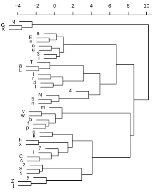
q G X a E e o u 3 i T 8 L l r d t 4 N 5 n m v w b f p g k h x 7 ! C c z S s y Z j

−4 −2 0 2 4 6 8 10

Figure 2: Sound similarities

• Pick one of the forty Swadesh concepts that has a corresponding word in both languages.

• Align these two words using the Levenshtein distance algorithm and store all alignment pairs.

This procedure was repeated 100,000 times. Of course most of the word pairs involved are not cognates, but it can be assumed in these cases, the alignments are largely random (except for univer-sal phonotactic patterns), such that genuine cog-nate alignments have a sufficiently large effect.

Note that language families vary considerably in size. While the data base comprises more than 1,000 Austronesian and more than 800 Niger-Congo languages, most families only consist of a handful of languages. As the procedure described above samples according to families rather than languages, languages that belong to small families are over-represented. This decision is intentional, because it prevents the algorithm from overfitting to the historically contingent properties of Aus-tronesian, Niger-Congo, and the few other large families.

Using weighted alignment, the similarity score for /hEnd/ ∼ /hant/ comes out as ≈ 4.1, while /hEnd/∼/mano/ has a score of≈0.2.

2.3 Language specific normalization

The second potential drawback of the LDND measure pertains to the second normalization step described above. The distances between trans-lation pairs are divided by the average distance between non-translation pairs. This serves to neutralize the impact of the sound inventories of the languages involved — the distances between languages with small and similar sound invento-ries are generally higher than those between lan-guages with large and/or different sound invento-ries.

Such a step is definitely necessary. However, dividing by the average distance does not take the effect of the variance of distances (or similarities) into account. If the distances between words from two languages have generally a low variance, the effect of cognacy among translation pairs is less visible than otherwise.

As an alternative, I propose the following simi-larity measure between words. Supposesis some independently defined similarity measure (such as the inverse normalized Levenshtein distance, or the Needleman-Wunsch similarity score). For simplicity’s sake, L1 and L2 are identified with

the set of words from the respective languages in the data base:

si(x, y|L1, L2)

.

=−log|{(x0,y0)∈L1×_|LL2|s(x0,y0)≥s(x,y)}|

1|×|L2|

The fraction gives the relative frequency of word pairs that are at least as similar to each other than x to y. If x and y are highly similar, this expression is close to 0. Conversely, if they are entirely dissimilar, the expression is close to 0.

The usage of the negative logarithm is mo-tivated by information theoretic considerations. Suppose you know a word x from L1 and you

have to pick out its translation from the words in L2. A natural search procedure is to start with

the word fromL2which is most similar tox, and

then to proceed according to decreasing similar-ity. The number of steps that this will take (or, up to a constant factor, the relative frequency of word pairs that are more similar to each other than x to its translation) is a measure of the distance

betweenxand its translation. Its logarithm corre-sponds (up to a constant factor) to the number of bits that you need to findx’s translation. Its nega-tion measures the amount of informanega-tion that you gain about some word if you know its translation in the other language.

The information theoretic similarity between two languages is defined as the average similar-ity between its translation pairs.

2.4 Comparison

These considerations lead to four different simi-larity/distance measures:

• based on Levenshtein distance vs. based on Needleman-Wunsch similarity score, and

• normalization via dividing by average score vs. information theoretic similarity measure.

To evaluate these measures, I defined a gold standard based on the know genetic affiliations of languages:

gs(L1, L2) =. 2ifL1andL2

belong to the same genus

gs(L1, L2) =. 1ifL1andL2

belong to the same family

but not the same genus gs(L1, L2) =. 0else

Three tests were performed for each metric. 2,000 different languages were picked at random and arranged into 1,000 pairs, and the four metrics were computed for each pair. First, the correlation of these metrics with the gold standard was com-puted. Second, a logistic regression model was fitted, where a language pair has the value 1 if the languages belong to the same genus, and 0 oth-erwise. Third, the same was repeated with fam-ilies rather than genera. In both cases, the log-likelihood of another sample of 1,000 language pairs according to the thus fitted models was com-puted.

metric correlation log-likelihood genus log-likelihood family

LDND −0.62 −116.0 −583.6

Levenshteini 0.61 −110.5 −530.5

NW normalized 0.62 −108.1 −518.5

NWi 0.64 −106.7 −514.5

Table 1: Tests of the different similarity measures

similarity metrics; only the absolute value mat-ters for the comparison), and it assigns the high-est log-likelihood on the thigh-est set both for family equivalence and for genus equivalence. We can thus conclude that this metric provides most in-formation about the genetic relationship between languages.

3 Visualization using CLANS

The pairwise similarity between all languages in the ASJP database (excluding creoles and artifi-cial languages) was computed according to this metric, and the resulting matrix was fed into CLANS. The outcome of two runs, using the same parameter settings, are given in Figure 3. Each circle represents one language. The circles are colored according to the genus affiliation of the corresponding language. Figure 4 gives the leg-end.

In both panels, the languages organize into clusters. Such clusters represent groups with a high mutual similarity. With few exceptions, all languages within such a cluster belong to the same genus. Obviously, some families (such as Aus-tronesian — shown in dark blue — and Indo-European — shown in brown — have a high co-herence and neatly correspond to a single com-pact cluster. Other families such as Australian — shown in light blue — and Niger-Congo — shown in red — are more scattered.

As can be seen from the two panels, the algo-rithm (which is initialized with a random state) may converge to different stable states with dif-ferent global configurations. For instance, Indo-European is located somewhere between Aus-tronesian, Sino-Tibetan — shown in yellow —, Trans-New-Guinea (gray) and Australian in the left panel, but between Austronesian, Austro-Asiatic (orange) and Niger-Congo (red) in the right panel. Nonetheless, some larger patterns are recurrent across simulations. For instance, the Tai-Kadai languages (light green) always end up

Figure 3: Languages of the world

in the proximity of the Austronesian languages. Likewise, the Nilo-Saharan languages (pink) do not always form a contiguous cluster, but they are always near the Niger-Congo languages.

It is premature to draw conclusions about deep genetic relationships from such observa-tions. Nonetheless, they indicate the presence of weak but non-negligible similarities between these families that deserve investigation. Visual-ization via CLANS is a useful tool to detect such weak signals in an exploratory fashion.

4 The languages of Eurasia

Working with all 5,000+ languages at once intro-duces a considerable amount of noise. In partic-ular the languages of the Americas and of Papua New Guinea do not show stable relationships to other language families. Rather, they are spread over the entire panel in a seemingly random fash-ion. Restricting attention to the languages of Eurasia (also including those Afro-Asiatic lan-guages that are spoken in Africa) leads to more pronounced global patterns.

In Figure 5 the outcome of two CLANS runs is shown. Here the global pattern is virtually iden-tical across runs (modulo rotation). The Dravid-ian languages (dark blue) are located at the cen-ter. Afro-Asiatic (brown), Uralic (pink), Indo-European (red), Sino-Tibetan (yellow), Hmong-Mien (light orange), Austro-Asiatic (orange), and Tai-Kadai (yellowish light green) are arranged

Figure 5: The languages of Eurasia

around the center. Japanese (light blue) is located further to the periphery outside Sino-Tibetan. Outside Indo-European the families Chukotko-Kamchatkan (light purple), Mongolic-Tungusic (lighter green), Turkic (darker green)3 Kartvelian (dark purple) and Yukaghir (pinkish) are fur-ther towards the periphery beyond the Turkic languages. The Caucasian languages (both the North Caucasian languages such as Lezgic and the Northwest-Caucasian languages such as Abk-haz) are located at the periphery somewhere be-tween Indo-European and Sino-Tibetan. Bu-rushaski (purple) is located near to the Afro-Asiatic languages.

Some of these pattern coincide with proposals about macro-families that have been made in the literature. For instance the relative proximity of Indo-European, Uralic, Chukotko-Kamchatkan, Mongolic-Tungusic, the Turkic languages, and Kartvelian is reminiscent of the hypothetical Nos-tratic super-family. Other patterns, such as the consistent proximity of Japanese to Sino-Tibetan, is at odds with the findings of historical linguis-tics and might be due to language contact. Other patterns, such as the affinity of Burushaski to the Afro-Asiatic languages, appear entirely puzzling.

3

According to the categorization used in ASJP, the Mon-golic, Tungusic, and Turkic languages form the genus Al-taic. This classification is controversial in the literature. In CLANS, Mongolic/Tungusic consistently forms a single cluster, and likewise does Turkic, but there is no indication that there is a closer relation between these two groups.

5 Conclusion

CLANS is a useful tool to aid automatic language classification. An important advantage of this software is its computational efficiency. Produc-ing a cluster map for a 5,000×5,000 similarity matrix hardly takes more than an hour on a reg-ular laptop, while it is forbidding to run a phy-logenetic tree algorithm with this hardware and this amount of data. Next to this practical ad-vantage, CLANS presents information in a format that facilitates the discovery of macroscopic pat-terns that are not easily discernible with alterna-tive methods. Therefore it is apt to be a useful addition to the computational toolbox of modern data-oriented historical and typological language research.

Acknowledgments

I would like to thank Andrei Lupas, David Er-schler, and Søren Wichmann for many inspiring discussions. Furthermore I am grateful for the comments I received from the reviewers for this workshop.

References

lexico-statistics: a combined approach to language classi-fication.Linguistic Typology, 13:167–179.

Tancred Frickey and Andrei N. Lupas. 2004. Clans: a java application for visualizing protein fami-lies based on pairwise similarity. Bioinformatics, 20(18):3702–3704.

Steven Henikoff and Jorja G. Henikoff. 1992. Amino acid substitution matrices from protein blocks. Pro-ceedings of the National Academy of Sciences, 89(22):10915–9.

Saul B. Needleman and Christian D. Wunsch. 1970. A general method applicable to the search for simi-larities in the amino acid sequence of two proteins.

Journal of Molecular Biology, 48:443453.

Jelena Prokic. 2010. Families and Resemblances. Ph.D. thesis, Rijksuniversiteit Groningen.