Mining Sentiments from Tweets

Mining Sentiments from Tweets

Akshat Bakliwal, Piyush Arora, Senthil Madhappan Nikhil Kapre, Mukesh Singh and Vasudeva Varma

Search and Information Extraction Lab,

International Institute of Information Technology, Hyderabad.

{akshat.bakliwal, piyush.arora}@research.iiit.ac.in,

{senthil.m, nikhil.kapre, mukeshkumar.singh}@students.iiit.ac.in, [email protected]

Abstract

Twitter is a micro blogging website, where users can post messages in very short text called Tweets. Tweets contain user opin-ion and sentiment towards an object or per-son. This sentiment information is very use-ful in various aspects for business and gov-ernments. In this paper, we present a method which performs the task of tweet sentiment identification using a corpus of pre-annotated tweets. We present a sentiment scoring func-tion which uses prior informafunc-tion to classify (binary classification ) and weight various sen-timent bearing words/phrases in tweets. Us-ing this scorUs-ing function we achieve classifi-cation accuracy of 87% on Stanford Dataset and 88% on Mejaj dataset. Using supervised machine learning approach, we achieve classi-fication accuracy of 88% on Stanford dataset.

1 Introduction

With enormous increase in web technologies, num-ber of people expressing their views and opinions via web are increasing. This information is very useful for businesses, governments and individuals. With over 340+ million Tweets (short text messages) per day, Twitter is becoming a major source of infor-mation.

Twitter is a micro-blogging site, which is popular because of its short text messages popularly known as “Tweets”. Tweets have a limit of 140 characters. Twitter has a user base of 140+ million active users1

1

As on March 21, 2012. Source:

http://en.wikipedia.org/wiki/Twitter

and thus is a useful source of information. Users often discuss on current affairs and share their per-sonals views on various subjects via tweets.

Out of all the popular social media’s like Face-book, Google+, Myspace and Twitter, we choose Twitter because 1) tweets are small in length, thus less ambigious; 2) unbiased; 3) are easily accessible via API; 4) from various socio-cultural domains.

In this paper, we introduce an approach which can be used to find the opinion in an aggregated col-lection of tweets. In this approach, we used two different datasets which are build using emoticons and list of suggestive words respectively as noisy la-bels. We give a new method of scoring “Popularity Score”, which allows determination of the popular-ity score at the level of individual words of a tweet text. We also emphasis on various types and levels of pre-processing required for better performance.

Roadmap for rest of the paper: Related work is discussed in Section 2. In Section 3, we describe our approach to address the problem of Twitter sentiment classification along with pre-processing steps.Datasets used in this research are discussed in Section 4. Experiments and Results are presented in Section 5. In Section 6, we present the feature vector approach to twitter sentiment classification. Section 7 presents as discussion on the methods and we con-clude the paper with future work in Section 8.

2 Related Work

Research in Sentiment Analysis of user generated content can be categorized into Reviews (Turney, 2002; Pang et al., 2002; Hu and Liu, 2004), Blogs (Draya et al., 2009; Chesley, 2006; He et al., 2008),

News (Godbole et al., 2007), etc. All these cat-egories deal with large text. On the other hand, Tweets are shorter length text and are difficult to analyse because of its unique language and struc-ture.

(Turney, 2002) worked on product reviews. Tur-ney used adjectives and adverbs for performing opinion classification on reviews. He used PMI-IR algorithm to estimate the semantic orientation of the sentiment phrase. He achieved an average accuracy of 74% on 410 reviews of different domains col-lected from Epinion. (Hu and Liu, 2004) performed feature based sentiment analysis. Using Noun-Noun phrases they identified the features of the products and determined the sentiment orientation towards each feature. (Pang et al., 2002) tested various ma-chine learning algorithms on Movie Reviews. He achieved 81% accuracy in unigram presence feature set on Naive Bayes classifier.

(Draya et al., 2009) tried to identify domain spe-cific adjectives to perform blog sentiment analysis. They considered the fact that opinions are mainly expressed by adjectives and pre-defined lexicons fail to identify domain information. (Chesley, 2006) per-formed topic and genre independent blog classifica-tion, making novel use of linguistic features. Each post from the blog is classified as positive, negative and objective.

To the best of our knowledge, there is very less amount of work done in twitter sentiment sis. (Go et al., 2009) performed sentiment analy-sis on twitter. They identified the tweet polarity us-ing emoticons as noisy labels and collected a train-ing dataset of 1.6 million tweets. They reported an accuracy of 81.34% for their Naive Bayes classi-fier. (Davidov et al., 2010) used 50 hashtags and 15 emoticons as noisy labels to create a dataset for twit-ter sentiment classification. They evaluate the effect of different types of features for sentiment extrac-tion. (Diakopoulos and Shamma, 2010) worked on political tweets to identify the general sentiments of the people on first U.S. presidential debate in 2008.

(Bora, 2012) also created their dataset based on noisy labels. They created a list of 40 words (pos-itive and negative) which were used to identify the polarity of tweet. They used a combination of a minimum word frequency threshold and Cate-gorical Proportional Difference as a feature

selec-tion method and achieved the highest accuracy of 83.33% on a hand labeled test dataset.

(Agarwal et al., 2011) performed three class (pos-itive, negative and neutral) classification of tweets. They collected their dataset using Twitter stream API and asked human judges to annotate the data into three classes. They had 1709 tweets of each class making a total of 5127 in all. In their research, they introduced POS-specific prior polarity features along with twitter specific features. They achieved max accuracy of 75.39% for unigram + senti fea-tures.

Our work uses (Go et al., 2009) and (Bora, 2012) datasets for this research. We use Naive Bayes method to decide the polarity of tokens in the tweets. Along with that we provide an useful insight on how preprocessing should be done on tweet. Our method of Senti Feature Identification and Popularity Score perform well on both the datasets. In feature vec-tor approach, we show the contribution of individual NLP and Twitter specific features.

3 Approach

Our approach can be divided into various steps. Each of these steps are independent of the other but important at the same time.

3.1 Baseline

In the baseline approach, we first clean the tweets. We remove all the special characters, targets (@), hashtags (#), URLs, emoticons, etc and learn the positive & negative frequencies of unigrams in train-ing. Every unigram token is given two probability scores: Positive Probability (Pp) and Negative

Prob-ability (Np) (Refer Equation 1). We follow the same

positive otherwise negative.

Pf = F requency in P ositive T raining Set

Nf = F requency in N egative T raining Set

Pp = P ositive P robability of the token.

= Pf/(Pf + Nf)

Np = N egative P robability of the token.

= Nf/(Pf + Nf)

(1)

3.2 Emoticons and Punctuations Handling

We make slight changes in the pre-processing mod-ule for handling emoticons and punctuations. We use the emoticons list provided by (Agarwal et al., 2011) in their research. This list2 is built from wikipedia list of emoticons3and is hand tagged into five classes (extremely positive, positive, neutral, negative and extremely negative). In this experi-ment, we replace all the emoticons which are tagged positive or extremely positive with ‘zzhappyzz’ and rest all other emoticons with ‘zzsadzz’. We append and prepend ‘zz’ to happy and sad in order to pre-vent them from mixing into tweet text. At the end, ‘zzhappyzz’ is scored +1 and ‘zzsadzz’ is scored -1. Exclamation marks (!) and question marks (?) also carry some sentiment. In general, ‘!’ is used when we have to emphasis on a positive word and ‘?’ is used to highlight the state of confusion or disagreement. We replace all the occurrences of ‘!’ with ‘zzexclaimzz’ and of ‘?’ with ‘zzquestzz’. We add 0.1 to the total tweet score for each ‘!’ and sub-tract 0.1 from the total tweet score for each ‘?’. 0.1 is chosen by trial and error method.

3.3 Stemming

We use Porter Stemmer4 to stem the tweet words. We modify porter stemmer and restrict it to step 1 only. Step 1 gets rid of plurals and -ed or -ing.

3.4 Stop Word Removal

Stop words play a negative role in the task of senti-ment classification. Stop words occur in both pos-itive and negative training set, thus adding more ambiguity in the model formation. And also, stop

2

http://goo.gl/oCSnQ

3

http://en.wikipedia.org/wiki/List of emoticons

4_{http://tartarus.org/ ˜martin/PorterStemmer/}

words don’t carry any sentiment information and thus are of no use to us. We create a list of stop words like he, she, at, on, a, the, etc. and ignore them while scoring. We also discard words which are of length≤2 for scoring the tweet.

3.5 Spell Correction

Tweets are written in random form, without any fo-cus given to correct structure and spelling. Spell correction is an important part in sentiment analy-sis of user- generated content. Users type certain characters arbitrary number of times to put more em-phasis on that. We use the spell correction algo-rithm from (Bora, 2012). In their algoalgo-rithm, they replace a word with any character repeating more than twice with two words, one in which the re-peated character is placed once and second in which the repeated character is placed twice. For example the word ‘swwweeeetttt’ is replaced with 8 words ‘swet’, ‘swwet’, ‘sweet’, ‘swett’, ‘swweet’, and so on.

Another common type of spelling mistakes oc-cur because of skipping some of characters from the spelling. like “there” is generally written as “thr”. Such types of spelling mistakes are not currently handled by our system. We propose to use phonetic level spell correction method in future.

3.6 Senti Features

At this step, we try to reduce the effect of non-sentiment bearing tokens on our classification sys-tem. In the baseline method, we considered all the unigram tokens equally and scored them using the Naive Bayes formula (Refer Equation 1). Here, we try to boost the scores of sentiment bearing words. In this step, we look for each token in a pre-defined list of positive and negative words. We use the list of of most commonly used positive and negative words provided by Twitrratr5. When we come across a to-ken in this list, instead of scoring it using the Naive Bayes formula (Refer Equation 1), we score the to-ken +/- 1 depending on the list in which it exist. All the tokens which are missing from this list went un-der step 3.3, 3.4, 3.5 and were checked for their oc-currence after each step.

3.7 Noun Identification

After doing all the corrections (3.3 - 3.6) on a word, we look at the reduced word if it is being converted to a Noun or not. We identify the word as a Noun word by looking at its part of speech tag in English WordNet(Miller, 1995). If the majority sense (most commonly used sense) of that word is Noun, we discard the word while scoring. Noun words don’t carry sentiment and thus are of no use in our experi-ments.

3.8 Popularity Score

This scoring method boosts the scores of the most commonly used words, which are domain specific. For example, happy is used predominantly for ex-pressing the positive sentiment. In this method, we multiple its popularity factor (pF) to the score of each unigram token which has been scored in the previous steps. We use the occurrence frequency of a token in positive and negative dataset to decide on the weight of popularity score. Equation 2 shows how the popularity factor is calculated for each to-ken. We selected a threshold 0.01 min support as the cut-off criteria and reduced it by half at every level. Support of a word is defined as the proportion of tweets in the dataset which contain this token. The value 0.01 is chosen such that we cover a large num-ber of tokens without missing important tokens, at the same time pruning less frequent tokens.

Pf = F requency in P ositive T raining Set

Nf = F requency in N egative T raining Set

if(Pf−Nf)>1000)

pF = 0.9;

elseif((Pf −Nf)>500)

pF = 0.8;

elseif((Pf −Nf)>250)

pF = 0.7;

elseif((Pf −Nf)>100)

pF = 0.5;

elseif((Pf −Nf <50))

pF = 0.1;

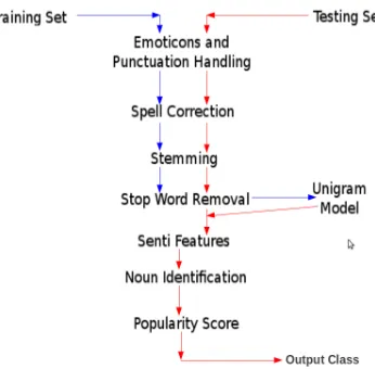
(2)

Figure 1 shows the flow of our approach.

Figure 1: Flow Chart of our Algorithm

4 Datasets

In this section, we explain the two datasets used in this research. Both of these datasets are built using noisy labels.

4.1 Stanford Dataset

This dataset(Go et al., 2009) was built automat-ically using emoticons as noisy labels. All the tweets which contain ‘:)’ were marked positive and tweets containing ‘:(’ were marked negative. Tweets that did not have any of these labels or had both were discarded. The training dataset has∼1.6 mil-lion tweets, equal number of positive and negative tweets. The training dataset was annotated into two classes (positive and negative) while the testing data was hand annotated into three classes (positive, neg-ative and neutral). For our experimentation, we use only positive and negative class tweets from the test-ing dataset for our experimentation. Table 1 gives the details of dataset.

Training Tweets

Positive 800,000

Negative 800,000

Total 1,600,000

Testing Tweets

Positive 180

Negative 180

Objective 138

Total 498

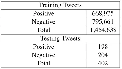
4.2 Mejaj

Mejaj dataset(Bora, 2012) was built using noisy la-bels. They collected a set of 40 words and manually categorized them into positive and negative. They label a tweet as positive if it contains any of the pos-itive sentiment words and as negative if it contains any of the negative sentiment words. Tweets which do not contain any of these noisy labels and tweets which have both positive and negative words were discarded.Table 2gives the list of words which were used as noisy labels. This dataset contains only two class data.Table 3gives the details of the dataset.

Positive Labels Negative Labels

amazed, amused, attracted, cheerful,

delighted, elated, excited, festive, funny,

hilarious, joyful, lively, loving, overjoyed, passion,

pleasant, pleased, pleasure, thrilled,

wonderful

annoyed, ashamed, awful, defeated,

depressed, disappointed,

discouraged, displeased, embarrassed, furious,

gloomy, greedy, guilty, hurt, lonely,

mad, miserable, shocked, unhappy,

upset

Table 2: Noisy Labels for annotating Mejaj Dataset

Training Tweets

Positive 668,975

Negative 795,661

Total 1,464,638

Testing Tweets

Positive 198

Negative 204

Total 402

Table 3: Mejaj Dataset

5 Experiment

In this section, we explain the experiments carried out using the above proposed approach.

5.1 Stanford Dataset

On this dataset(Go et al., 2009), we perform a series of experiments. In the first series of experiments,

we train on the given training data and test on the testing data. In the second series of experiments, we perform 5 fold cross validation using the training data. Table 4shows the results of each of these ex-periments on steps which are explained in Approach (Section 3).

In table 4, we give results for each step emoticons and punctuations handling, spell correction, stem-ming and stop word removal mentioned in Approach Section (Section 3). The Baseline + All Combined results refers to combination of these steps (emoti-cons, punctuations, spell correction, Stemming and stop word removal) performed together. Series 2 re-sults are average of accuracy of each fold.

5.2 Mejaj Dataset

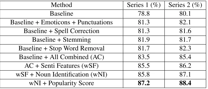
Similar series of experiments were performed on this dataset(Bora, 2012) too. In the first series of experiments, training and testing was done on the respective given datasets. In the second series of ex-periments, we perform 5 fold cross validation on the training data. Table 5 shows the results of each of these experiments.

In table 5, we give results for each step emoticons and punctuations handling, spell correction, stem-ming and stop word removal mentioned in Approach Section (Section 3). The Baseline + All Combined results refers to combination of these steps (emoti-cons, punctuations, spell correction, Stemming and stop word removal) performed together. Series 2 re-sults are average of accuracy of each fold.

5.3 Cross Dataset

To validate the robustness of our approach, we ex-perimented with cross dataset training and testing. We trained our system on one dataset and tested on the other dataset. Table 6reports the results of cross dataset evaluations.

6 Feature Vector Approach

Method Series 1 (%) Series 2 (%)

Baseline 78.8 80.1

Baseline + Emoticons + Punctuations 81.3 82.1

Baseline + Spell Correction 81.3 81.6

Baseline + Stemming 81.9 81.7

Baseline + Stop Word Removal 81.7 82.3

Baseline + All Combined (AC) 83.5 85.4

AC + Senti Features (wSF) 85.5 86.2

wSF + Noun Identification (wNI) 85.8 87.1

wNI + Popularity Score 87.2 88.4

Table 4: Results on Stanford Dataset

Method Series 1 (%) Series 2 (%)

Baseline 77.1 78.6

Baseline + Emoticons + Punctuations 80.3 80.4

Baseline + Spell Correction 80.1 80.0

Baseline + Stemming 79.1 79.7

Baseline + Stop Word Removal 80.2 81.7

Baseline + All Combined (AC) 82.9 84.1

AC + Senti Features (wSF) 86.8 87.3

wSF + Noun Identification (wNI) 87.6 88.2

wNI + Popularity Score 88.1 88.1

Table 5: Results on Mejaj Dataset

Method Training Dataset Testing Dataset Accuracy

wNI + Popularity Score Stanford Mejaj 86.4%

wNI + Popularity Score Mejaj Stanford 84.7%

Table 6: Results on Cross Dataset evaluation

NLP Unigram (f1) # of positive and negative unigram

Bigram (f2) # of positive and negative Bigram

Twitter Specific

Hashtags (f3) # of positive and negative hashtags Emoticons (f4) # of positive and negative emoticons

URLs (f5) Binary Feature - presence of URLs Targets (f6) Binary Feature - presence of Targets Special Symbols (f7) Binary Feature - presence of ‘!’

Feature Set Accuracy (Stanford)

f1 + f2 85.34%

f3 + f4 + f7 53.77%

f3 + f4 + f5 + f6 + f7 60.12% f1 + f2 + f3 + f4 + f7 85.89%

f1 + f2 + f3 + f4 +

f5 + f6 + f7 87.64%

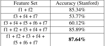
Table 8: Results of Feature Vector Classifier on Stanford Dataset

unigrams matched, negative unigrams matched, pos-itive bigrams matched, negative bigrams matched, etc and Twitter specific features included Emoti-cons, Targets, HashTags, URLs, etc. Table 7shows the features we have considered.

HashTags polarity is decided based on the con-stituent words of the hashtags. Using the list of pos-itive and negative words from Twitrratr6, we try to find if hashtags contains any of these words. If so, we assign the polarity of that to the hashtag. For example, “#imsohappy” contains a positive word “happy”, thus this hashtag is considered as posi-tive hashtag. We use the emoticons list provided by (Agarwal et al., 2011) in their research. This list7 is built from wikipedia list of emoticons8 and is hand tagged into five classes (extremely positive, positive, neutral, negative and extremely negative). We reduce this five class list to two class by merging extremely positive and positive class to single posi-tive class and rest other classes (extremely negaposi-tive, negative and neutral) to single negative class. Ta-ble 8reports the accuracy of our machine learning classifier on Stanford dataset.

7 Discussion

In this section, we present a few examples evaluated using our system. The following example denotes the effect of incorporating the contribution of emoti-cons on tweet classification. Example“Ahhh I can’t move it but hey w/e its on hell I’m elated right now :-D”. This tweet contains two opinion words, “hell” and “elated”. Using the unigram scoring method, this tweet is classified neutral but it is actually

posi-6

http://twitrratr.com/

7

http://goo.gl/oCSnQ

8_{http://en.wikipedia.org/wiki/List of emoticons}

tive. If we incorporate the effect of emoticon “:-D”, then this tweet is tagged positive. “:-D” is a strong positive emoticon.

Consider this example, “Bill Clinton Fail -Obama Win?”. In this example, there are two senti-ment bearing words, “Fail” and “Win”. Ideally this tweet should be neutral but this is tagged as a posi-tive tweet in the dataset as well as using our system. In this tweet, if we calculate the popularity factor (pF) for “Win” and “Fail”, they come out to be 0.9 and 0.8 respectively. Because of the popularity fac-tor weight, the positive score domniates the negative score and thus the tweet is tagged as positive. It is important to identify the context flow in the text and also how each of these words modify or depend on the other words of the tweet.

For calculating the system performance, we as-sume that the dataset which is used here is correct. Most of the times this assumption is true but there are a few cases where it fails. For example, this tweet “My wrist still hurts. I have to get it looked at. I HATE the dr/dentist/scary places. :( Time to watch Eagle eye. If you want to join, txt!” is tagged as positive, but actually this should have been tagged negative. Such erroneous tweets also effect the sys-tem performance.

There are few limitations with the current pro-posed approach which are also open research prob-lems.

1. Spell Correction: In the above proposed ap-proach, we gave a solution to spell correction which works only when extra characters are en-tered by the user. It fails when users skip some characters like “there” is spelled as “thr”. We propose the use of phonetic level spell correc-tion to handle this problem.

2. Hashtag Segmentation: For handling hashtags, we looked for the existence of the positive or negative words9 in the hashtag. But there can be some cases where it may not work correctly. For example, “#thisisnotgood”, in this hashtag if we consider the presence of positive and neg-ative words, then this hashtag is tagged posi-tive (“good”). We fail to capture the presence and effect of “not” which is making this

tag as negative. We propose to devise and use some logic to segment the hashtags to get cor-rect constituent words.

3. Context Dependency: As discussed in one of the examples above, even tweet text which is limited to 140 characters can have context de-pendency. One possible method to address this problem is to identify the objects in the tweet and then find the opinion towards those objects.

8 Conclusion and Future Work

Twitter sentiment analysis is a very important and challenging task. Twitter being a microblog suffers from various linguistic and grammatical errors. In this research, we proposed a method which incorpo-rates the popularity effect of words on tweet senti-ment classification and also emphasis on how to pre-process the Twitter data for maximum information extraction out of the small content. On the Stanford dataset, we achieved 87% accuracy using the scor-ing method and 88% usscor-ing SVM classifier. On Me-jaj dataset, we showed an improvement of 4.77% as compared to their (Bora, 2012) accuracy of 83.33%. In future, This work can be extended through in-corporation of better spell correction mechanisms (may be at phonetic level) and word sense disam-biguation. Also we can identify the target and enti-ties in the tweet and the orientation of the user to-wards them.

Acknowledgement

We would like to thank Vibhor Goel, Sourav Dutta and Sonil Yadav for helping us with running SVM classifier on such a large data.

References

Agarwal, A., Xie, B., Vovsha, I., Rambow, O. and Pas-sonneau, R. (2011). Sentiment analysis of Twitter

data. In Proceedings of the Workshop on Languages in Social Media LSM ’11.

Bora, N. N. (2012). Summarizing Public Opinions in Tweets. In Journal Proceedings of CICLing 2012, New Delhi, India.

Chesley, P. (2006). Using verbs and adjectives to auto-matically classify blog sentiment. In In Proceedings of AAAI-CAAW-06, the Spring Symposia on Compu-tational Approaches.

Davidov, D., Tsur, O. and Rappoport, A. (2010). En-hanced sentiment learning using Twitter hashtags and smileys. In Proceedings of the 23rd International Con-ference on Computational Linguistics: Posters COL-ING ’10.

Diakopoulos, N. and Shamma, D. (2010). Characterizing debate performance via aggregated twitter sentiment. In Proceedings of the 28th international conference on Human factors in computing systems ACM.

Draya, G., Planti, M., Harb, A., Poncelet, P., Roche, M. and Trousset, F. (2009). Opinion Mining from Blogs. In International Journal of Computer Informa-tion Systems and Industrial Management ApplicaInforma-tions (IJCISIM).

Go, A., Bhayani, R. and Huang, L. (2009). Twitter Sen-timent Classification using Distant Supervision. In CS224N Project Report, Stanford University.

Godbole, N., Srinivasaiah, M. and Skiena, S. (2007). Large-Scale Sentiment Analysis for News and Blogs. In Proceedings of the International Conference on We-blogs and Social Media (ICWSM).

He, B., Macdonald, C., He, J. and Ounis, I. (2008). An effective statistical approach to blog post opinion re-trieval. In Proceedings of the 17th ACM conference on Information and knowledge management CIKM ’08. Hu, M. and Liu, B. (2004). Mining Opinion Features in

Customer Reviews. In AAAI.

Miller, G. A. (1995). WordNet: A Lexical Database for English. Communications of the ACM 38, 39–41. Pang, B., Lee, L. and Vaithyanathan, S. (2002). Thumbs

up? Sentiment Classification using Machine Learning Techniques.