Complex dynamics emerging in Rule 30 with majority memory

Martinez, G. J., Adamatzky, A., Alonso-Sanz, R. and Mora, J. C. (2010) Complex dynamics emerging in Rule 30 with majority mem-ory. Complex Systems, 18 (3). pp. 345-365. ISSN 0891-2513 Avail-able from: http://eprints.uwe.ac.uk/10410

We recommend you cite the published version. The publisher’s URL is:

http://www.complex-systems.com/Archive/hierarchy/abstract.cgi?vol=18&iss=3&art=05

Refereed: Yes (no note)

Disclaimer

UWE has obtained warranties from all depositors as to their title in the material deposited and as to their right to deposit such material.

UWE makes no representation or warranties of commercial utility, title, or fit-ness for a particular purpose or any other warranty, express or implied in respect of any material deposited.

Martinez, G. J., Adamatzky, A., Alonso-Sanz, R. and Mora, J. C. (2010) Complex dynamics emerging in Rule 30 with majority mem-ory. Complex Systems, 18 (3). pp. 345-365. ISSN 0891-2513 Avail-able from: http://eprints.uwe.ac.uk/10410

We recommend you cite the published version. The publisher’s URL is:

http://www.complex-systems.com/Archive/hierarchy/abstract.cgi?vol=18&iss=3&art=05

Refereed: Yes (no note)

Disclaimer

UWE has obtained warranties from all depositors as to their title in the material deposited and as to their right to deposit such material.

UWE makes no representation or warranties of commercial utility, title, or fit-ness for a particular purpose or any other warranty, express or implied in respect of any material deposited.

Complex Dynamics Emerging in Rule 30

with Majority Memory

Genaro J. Martínez* H1,2L Andrew Adamatzky H1L Ramon Alonso-Sanz H1L

H1L_{Department of Computer Science} University of the West of England Bristol BS16 1QY, United Kingdom

H2L_{Instituto de Ciencias Nucleares and Centro de Ciencias de la Complejidad} Universidad Nacional Autónoma de México

*[email protected] Juan C. Seck-Tuoh-Mora

Centro de Investigación Avanzada en Ingeniería Industrial Universidad Autónoma del Estado de Hidalgo Pachuca Hidalgo, México

In cellular automata (CAs) with memory, the unchanged maps of conventional CAs are applied to cells endowed with memory of their past states in some specified interval. We implement the rule 30 automa-ton and show that by using the majority memory function we can trans-form the quasi-chaotic dynamics of classical rule 30 into domains of traveling structures with predictable behavior. We analyze morphologi-cal complexity of the automata and classify glider dynamics (particle, self-localizations) in the memory-enriched rule 30. Formal ways of encoding and classifying glider dynamics using de Bruijn diagrams, soli-ton reactions, and quasi-chemical representations are provided.

1. Introduction

An elementary cellular automaton (CA) is a one-dimensional array of finite automata, where each automaton takes two states and updates its state in discrete time depending on its own state and the states of its two closest neighbors. All cells update their state synchronously. The following general classification of elementary CAs was intro-duced in [1].

Class I. CAs evolve to a homogeneous state.

Class II. CAs that evolve periodically.

Class III. CAs that evolve chaotically.

Class IV. Include all previous cases, also known as the class of complex rules.

Class IV is of particular interest because the rules exhibit nontrivial behavior with rich and diverse patterns, as shown for rule 54 in [2, 3].

2. Basic Notation

2.1 One-Dimensional Cellular Automata

One-dimensional CAs are represented by an infinite array of cells x_i where iœ and each x takes a value from a finite alphabet S. Thus, a sequence of cells 8x_i< of finite length n represents a string or global configuration c on S with the set of finite configurations represented as Sn. An evolution is represented by a sequence of configurations 9ci= given by the mapping F:SnØ Sn; thus their global relation is provided as

(1)

FIctMØct+1

where t is time and every global state of c is defined by a sequence of cell states. Also, the cell states in configuration ct are updated at the next configuration ct+1 simultaneously by a local function j:

(2)

jIx_it_-r, … ,x_it, … ,x_it_+rMØx_it+1.

Wolfram represents a one-dimensional CA with two parameters

Hk,rL where k†S§ is the number of states, and r is the neighborhood radius. Elementary CAs are defined by parameters Hk2,r1L. There are Sn different neighborhoods (where n2r+1) and kkn different evolution rules.

We used automata with periodic boundary conditions in our computer experiments.

2.2 Cellular Automata with Memory

Conventional CAs are ahistoric (memoryless): that is, the new state of a cell depends on the neighborhood configuration solely at the preced-ing time step of j as in equation (2).

Cellular automata with memory consider an extension to the stan-dard CA framework by implementing memory capabilities in cells x_i from its own history.

Thus, to implement memory we incorporate a memory function f,

(3)

fIx_it-t, … ,xt_i-1,x_itMØs_i

such that t <t determines the degree of memory backward and each cell s_iœ S is a state function of the series of states of the cell x_i with memory up to the current time step. Finally, to execute the evolution we apply the original rule as:

jI… ,s_it_-1,s_it,s_it₊₁, …MØx_it+1.

Thus, in CAs with memory, while the mappings j remain unal-tered, historic memory of all past iterations is retained by featuring each cell with a summary of its past states from f. Therefore, cells

canalize memory to the map j.

346 G. J. Martínez et. al

Thus, in CAs with memory, while the mappings j remain unal-tered, historic memory of all past iterations is retained by featuring each cell with a summary of its past states from f. Therefore, cells

canalize memory to the map j.

As an example, we define the majority memory as

(4)

f_majØs_i

where, in case of a tie given by S₁S₀ from f, we will take the last value x_i. So the f_maj function represents the classic majority function

[4] on the cells Ix_it-t, … ,x_it-1,x_itM and defines a temporal ring before finally getting the next global configuration c.

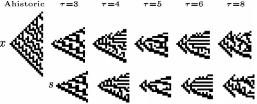
Figure 1. The effect of majority memory with increasing depths on rule 30 starting from a single site live cell.

Majority memory exerts a general inertial effect [5]. This effect, when starting from a single site live cell, notably restrains the dynam-ics, as illustrated using rule 30 in Figure 1. This figure shows the spatio-temporal patterns of both the current x state values and that of the underlying s values.

3. Elementary Cellular Automaton Rule 30

Rule 30 was initially studied by Wolfram in [1] because of its chaotic global behavior while looking for a random number generator. Rule°30 is an elementary CA that evolves in one dimension of order

H2, 1L. An interesting property is that it has a surjective relation and thus does not have Garden of Eden configurations [6]. In this way, any configuration always has at least one predecessor.

Here is the local rule j corresponding to rule 30:

j_R30 1 if 100, 011, 010, 001

0 if 111, 110, 101, 000.

Generally speaking, rule 30 displays a typical chaotic global behav-ior, that is, it is in Wolfram’s Class III. An interesting study on rule 30 showing a local nested structure that repeats periodically while look-ing for invertible properties is given in [7].

Complex Dynamics Emerging in Rule 30 with Majority Memory 347

Generally speaking, rule 30 displays a typical chaotic global behav-ior, that is, it is in Wolfram’s Class III. An interesting study on rule 30 showing a local nested structure that repeats periodically while look-ing for invertible properties is given in [7].

So, initially j_R30 has a 50% probability of states zero or one, and consequently each state appears with the same frequency.

HaL HbL

Figure 2. (a) Typical behavior of rule 30, where a single cell in state one leads to a chaotic state. (b) Shows the automaton behavior from a random initial condition with an initial density of 50% for each state. Both automata evolved on a ring of 497 cells (with a periodic boundary property) to 417 generations. White cells represent state zero and dark cells the state one.

Also, the evolution of rule 30 presents the following feature: if an initial configuration is covered all in state one, then it always evolves into one; but if this is empty or filled with state one then this always evolves to state zero. Figure 2 shows two typical cases of evolution with rule 30.

3.1 De Bruijn and Subset Diagrams in Rule 30

Given a finite sequence wœ Sm, such that ww₁, … ,wm, let

aHwLw₁, bHwLw₂, … ,wm, and yHwLw1, … ,wm-1. With these elements, we can specify a labeled directed graph known as a de Bruijn diagram  8N;E< associated with the evolution rule of the CA. The nodes of  are defined by NS2r _{and the set of directed} edges EŒ S2r_äS2r _{is defined as}

(5) E8Hv,wL v,wœN, bHvLyHwL<.

For every directed edge Hv,wLœE, let hHv,wLa wœ S2r+1

where aaHvL; that is, hHv,wL is a neighborhood of the automaton. In this way, the edge Hv,wL is labeled by jÈhHv,wL; hence, every labeled path in  represents the evolution of the corresponding sequence specified by its nodes. Since each wœN can be described by a number base k of length 2r, every node in  can be enumerated by a unique element in _k2r, which is useful for simplifying the diagram.

The de Bruijn diagram associated with rule 30 is depicted in Figure 3, where black edges indicate the neighborhoods evolving into zero and those evolving into one are shown by gray edges. The de Bruijn and subset diagrams were calculated using NXLCAU21 designed by McIn-tosh. The program is available from delta.cs.cinvestav.mx/~mcinMcIn-tosh.

348 G. J. Martínez et. al

For every directed edge Hv,wLœE, let hHv,wLa wœ S2r+1

where aaHvL; that is, hHv,wL is a neighborhood of the automaton. In this way, the edge Hv,wL is labeled by jÈhHv,wL; hence, every labeled path in  represents the evolution of the corresponding sequence specified by its nodes. Since each wœN can be described by a number base k of length 2r, every node in  can be enumerated by a unique element in _k2r, which is useful for simplifying the diagram.

The de Bruijn diagram associated with rule 30 is depicted in Figure 3, where black edges indicate the neighborhoods evolving into zero and those evolving into one are shown by gray edges. The de Bruijn and subset diagrams were calculated using NXLCAU21 designed by McIn-tosh. The program is available from delta.cs.cinvestav.mx/~mcinMcIn-tosh.

Figure 3. De Bruijn diagram for the elementary CA rule 30.

Figure 3 shows that there are four neighborhoods evolving into zero and four into one, meaning that each state has the same probabil-ity to appear during the evolution. This indicates the possibilprobabil-ity that the automaton is surjective, that is, there are no Garden of Eden configurations. Classical analysis in graph theory has been applied over de Bruijn diagrams for studying topics such as reversibility [8]; cycles in the diagram indicate periodic elements in the evolution of the automaton if the label of the cycle corresponds to the sequence defined by its nodes, in periodic boundary conditions. The cycles in the de Bruijn diagram from Figure 3 are presented in Figure 4.

Figure 4. Cycles in the de Bruijn diagram and the corresponding periodic evolution for cycle H1, 2L.

The largest cycle in Figure 4 indicates that the undefined repetition of sequence w_b10 establishes a periodic structure without displace-ment in one generation during the evolution of rule 30. We then say that w_b is the filter in rule 30. A filter is a periodic sequence that exists alone or in blocks during the evolution; thus, suppressing such a string produces a new view. In the present paper, we apply the filter to the original rule 30 and its modifications with memory. Thus, we can see how a de Bruijn diagram can recognize any periodic structures in a CA [3, 9].

Complex Dynamics Emerging in Rule 30 with Majority Memory 349

The largest cycle in Figure 4 indicates that the undefined repetition of sequence w_b10 establishes a periodic structure without displace-ment in one generation during the evolution of rule 30. We then say that w_b is the filter in rule 30. A filter is a periodic sequence that exists alone or in blocks during the evolution; thus, suppressing such a string produces a new view. In the present paper, we apply the filter to the original rule 30 and its modifications with memory. Thus, we can see how a de Bruijn diagram can recognize any periodic structures in a CA [3, 9].

A de Bruijn diagram is nondeterministic in the sense that a given node may have several output edges with the same label. A classical approach to analyzing the diagram would be to construct the subset (or power) diagram in order to obtain a deterministic version for the de Bruijn diagram in the evolution rule [10, 11].

The subset diagram is defined as  8,< where  8P PŒ S‹«< is the set of nodes of  and the directed edges are defined by Õä where for P₁,P₂œ there is a directed edge

HP₁,P₂L labeled by aœS in  if and only if P₂ is the maximum subset such that for every cœP₂ there exists bœP₁ such that jHb,cLa.

The inclusion of the empty set assures that every edge has a well-defined ending node. For a CA with k states, it is fulfilled that

†§2k2r, which implies an exponential growth in the number of nodes in  when more states are considered. Every Pœ can be iden-tified by a binary number showing the states belonging to this subset, that is, taking the states as an ordered list. The states in P can be signed by a 1 and the others by 0, making a unique binary sequence to identify the subset. The decimal value of this binary number can be taken to get a shorter representation where the empty set has a deci-mal number 0 and the full subset pS has the number 2k2r-1. The subset diagram corresponding to rule 30 is shown in Figure 5.

Figure 5. Subset diagram for rule 30.

In Figure 5, the subset diagram has no path starting from the full subset (node 15) going to the empty subset (node 0). This means that every sequence can be produced by the evolution of the automaton and there are no Garden of Eden sequences. Thus, the automaton is surjective. The subset diagram can also be used as a deterministic automaton for calculating ancestors of any desired sequence [12] by recognizing the regular expressions that may be generated by the corresponding automaton. Some of these expressions would be able to represent interesting structures as gliders [13]; however, more effort is needed in order to get a straightforward detection of such constructions in the diagram.

350 G. J. Martínez et. al

In Figure 5, the subset diagram has no path starting from the full subset (node 15) going to the empty subset (node 0). This means that every sequence can be produced by the evolution of the automaton and there are no Garden of Eden sequences. Thus, the automaton is surjective. The subset diagram can also be used as a deterministic automaton for calculating ancestors of any desired sequence [12] by recognizing the regular expressions that may be generated by the corresponding automaton. Some of these expressions would be able to represent interesting structures as gliders [13]; however, more effort is needed in order to get a straightforward detection of such constructions in the diagram.

Finally, such diagrams help get periodic strings that eventually represent a general filter w_b working on the original rule 30 and rule 30 with memory. Also, we will take advantage of these results to find gliders in the strings.

4. Majority Memory Helps to Discover Complex Dynamics in Rule 30

This section reports on how the majority memory f helps in the discovery of complex dynamics in elementary CAs by experimenta-tion. For an introduction to elementary CAs with memory, see [14|16].

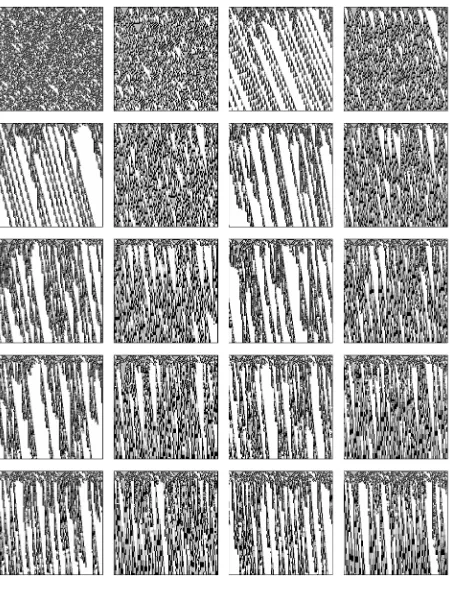
Figure 6 displays different scenarios where the majority memory

f_maj works on rule 30 to extract the complex dynamics. The evolu-tions should be read from left to right and up to down. All of these evolutions use the same random initial density and filter w_b (including the original rule 30). Thus, the first evolution shown in Figure 6 is the original rule 30, that is, without majority memory. In the original evolution we can see gaps that the filter can clean. Tradi-tionally, it was difficult to distinguish such a filter, but when f_maj was applied to rule 30 its presence was more evident. A general technique for getting filters was developed by Wuensche in [17].

Initially, even values of t seem to extract gliders more quickly and odd values fight to reach an order. Eventually, the majority memory will converge to one stability in F while t increases.

The first snapshot calculating f_maj with t3 is shown by the second evolution in Figure 6. It is not yet clear how memory induces another behavior because the global behavior is still similar to the original with only small changes.

On the other hand, the third evolution with t4 does extract peri-odic patterns. The evolution might not display impressive gliders but it already allows picking out more diversity in mobile localizations on lattices of 100ä100 cells. Thus, we have enumerated and ordered values of t from Figure 6 based on the space-time dynamics they are responsible for:

Chaotic global behavior: t0, 3, 5, 7, 9, 11, 13, 15, 17, 19, 21

Periodic patterns: t4, 6, 8, 10, 12, 14, 16, 18, 19, 20, 21

Collision patterns: t6, 8, 10, 12

Complex Dynamics Emerging in Rule 30 with Majority Memory 351

Figure 6. Complex dynamics emerging in rule 30 with majority memory f_maj

from a range of values from t3 to t21. The first evolution shows the original function. Evolutions were calculated on a ring of 104 cells in 104 generations with a random initial density of 50% and the same initial conditions were used in all cases. Also, the filter w_b was applied to clearly show the structures.

4.1 Morphological Complexity in Rule 30 with Memory

In this section we explore some techniques for finding global complex dynamics in rule 30 with and without majority memory.

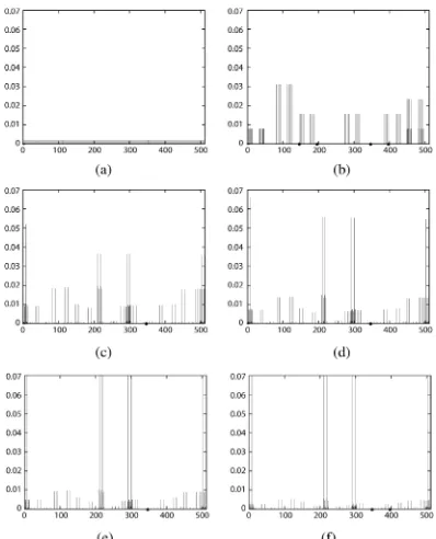
We evaluate the morphological complexity of a CA using the morphological richness approach in [18]. We calculate the statistical morphological richness m as follows. Given the space-time configura-tion of a one-dimensional CA, we extract the 3ä3 cell neighborhood state for each site of the configuration and build a distribution of the neighborhood states over an extended period of the automaton’s development time.

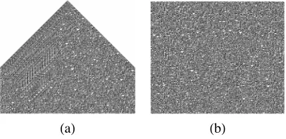
Examples of morphological richness m are shown in Figure 7. A control case, where the next state of a cell is calculated at random from the distribution of space-time neighborhood states, is uniform (Figure 7(a)). Two-dimensional random configurations are morpho-logically rich. The morphology of memoryless, classical rule 30 is characterized by few peaks in the local domain distributions, where several space-time templates dominate in the global space-time config-uration (Figure 7(b)). The statistical morphological richness m

decreases.

352 G. J. Martínez et. al

Examples of morphological richness m are shown in Figure 7. A control case, where the next state of a cell is calculated at random from the distribution of space-time neighborhood states, is uniform (Figure 7(a)). Two-dimensional random configurations are morpho-logically rich. The morphology of memoryless, classical rule 30 is characterized by few peaks in the local domain distributions, where several space-time templates dominate in the global space-time config-uration (Figure 7(b)). The statistical morphological richness m

decreases.

Incorporating memory in the cell-state transition rules leads to an erosion of the distribution (Figure 7(c)) and thus slight increases in m. With an increase in the memory depth, the shape of the morphologi-cal distribution changes just slightly, up to minor height variations in the major peaks (Figures 7(d) through (f)).

Figure 7. Morphological richness. Cellular automaton length of 1500 cells with a running time of 5000 steps. (a) Random update of cell states. (b) Rule 30 without memory. Rule 30 with memory: (c) t3, (d) t5, (e) t10, and (f) t21.

The number r of 3ä3 blocks (of states 0 and 1) that never appear in the space-time configuration of a CA can be used to express an estimate of the nominal morphological richness; smaller r indicate a richer nominal configuration.

The difference between statistical m and nominal r measures of morphological richness is that m allows picking most common configurations of local domains, while r just shows how many blocks of 3ä3 states appeared in the automaton evolution at least once.

For the case of randomly updating cell states, all blocks are present in the space-time configuration and r0.

Complex Dynamics Emerging in Rule 30 with Majority Memory 353

For the case of randomly updating cell states, all blocks are present in the space-time configuration and r0.

Memoryless automata governed by rule 30 have r434 so the total number of possible blocks is 512. When memory is first incorporated into the cell-state transition function, richness decreases, for example, with t1 we have r448. Then we observe a consistent increase in complexity. Thus, rule 30 with small-depth memory (t2) r140, drastically decreases to r68 for t3. The richness is stabilized, or rather oscillates around r values of 20 to 40 with a further increase of memory.

In summary, we found that majority memory increases the nominal complexity of a CA but decreases its statistical complexity.

4.2 Gliders in Rule 30 with Memory t8

Most frequently the complex dynamics of an elementary CA is related to gliders, glider guns, and nontrivial reactions between localizations, for example, rules 110 or 54 [2, 19]. The phenomena, and their regu-lar expressions [3, 9], may lead to the discovery of novel systems with computational universality [20, 21].

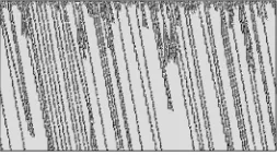
Figure 8. Gliders emerging in rule 30 with f_maj and t8. This evolution shows how some kinds of gliders arise and still interact from random initial conditions. The evolution was calculated on a ring of 590 cells to 320 genera-tions, with an initial density of 50%.

Among the sets of complex dynamics in rule 30 determined by t

(shown in Figure 6), we have chosen the memory f_maj with t8. In this way, Figure 8 illustrates an ample evolution space of its global dynamics.

Of course, these gliders may not be as impressive as others from such well-known complex rules as 110, 54, or some other one-dimen-sional rules [1, 2, 19, 22, 23]. However, it is interesting that f_maj is able to open complex patterns from chaotic rules.

Nevertheless, even though rule 30 does not offer an ample range of complex dynamics, it is useful for describing gliders and collisions. So, we shall illustrate how a chaotic CA can be decomposed as a complex system.

354 G. J. Martínez et. al

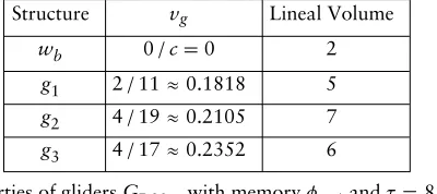
Figure 9. Set of gliders G_R30m with memory f_maj and t8.

We now classify the family of gliders and enumerate some of their properties. Figure 9 displays the family of gliders G_R30m9g₁,g₂,g₃=. As was hoped, an immediate consequence is that gliders in CAs with memory have longer periods.

Structure vg Lineal Volume

w_b 0êc 0 2

g₁ 2ê11º0.1818 5

g₂ 4ê19º0.2105 7

g₃ 4ê17º0.2352 6

Table 1. Properties of gliders G_R30m with memory f_maj and t8.

Table 1 summarizes the basic properties of each glider. Practically, all gliders in this domain have a constant displacement of four cells to the right and no glider with speed zero was found, and yet finding a glider gun in this domain is more complicated. Nevertheless, some interesting reactions did originate from G_R30m.

Structure w_b does not have a displacement and it is also not a glider. This pattern is the periodic background in rule 30 and repre-sents the filter. It was really hard to detect the existence of a periodic background evolving from the original rule. But when f_maj was applied, a periodic pattern began to emerge that was inherited from

j_R30. Finally, this filter was confirmed with its respective de Bruijn and cycle diagrams (see Section 3.1).

4.3 Reactions between Gliders from G_R30m

We now demonstrate some simple examples of collisions between glid-ers. Codes for all gliders, necessary to generate the whole set of binary collisions, are presented in the Appendix.

Complex Dynamics Emerging in Rule 30 with Majority Memory 355

Figure 10 shows how a stream of g₁ gliders is deleted from a reaction cycle:

g₃+g₁Øg₂andg₂+g₁Øg₃.

Figure 10. Deleting streams of g₁ gliders initialized with a single g₃ glider.

To obtain such a cycle by glider reactions, we can code an unlim-ited initial condition as ...g₃...g₁ ....g₁ ....g₁.... , that can be reduced as ...g₃...g₁H....g₁L* (where a dot represents a copy of w_b). Finally, the evolution produces the given cycle, with nine periods of g₃ and eight periods of g₂. Thus, each column presents 1135, 2270, and 3405 generations, respectively. In such a representation, codes of gliders will be different from codes used in our previous papers [3, 9, 19]. The glider reactions were produced using the OSXLCAU21 system available at uncomp.uwe.ac.uk/ genaro/OSXCASystems.html.

Since the better way to preserve j_R30 and f_maj is to code the glid-ers as “natural”, we consider the codification from its original initial condition. See Appendix B where some strings are defined to get glid-ers with memory from their original functions.

HaL HbL HcL

Figure 11. Some simple reactions display how to (a) delete, (b) read, and (c)

preserve information with gliders using rule 30 with memory.

Some simple but interesting reactions from G_R30m are illustrated in Figure 11. The first reaction shows the annihilation of gliders g₂ and g₁. The second reaction shows how a transformation g₃ glider trans-forms a g₁ glider into a g₂. The third reaction shows a soliton-like collision between gliders g₂ and g₁. The soliton reaction between glid-ers is particularly promising because it can be used to implement computation, for example, as in the carry-ripple adder embedded by phase coding solitons in parity CAs [24, 25].

356 G. J. Martínez et. al

Some simple but interesting reactions from G_R30m are illustrated in Figure 11. The first reaction shows the annihilation of gliders g₂ and g₁. The second reaction shows how a transformation g₃ glider trans-forms a g₁ glider into a g₂. The third reaction shows a soliton-like collision between gliders g₂ and g₁. The soliton reaction between glid-ers is particularly promising because it can be used to implement computation, for example, as in the carry-ripple adder embedded by phase coding solitons in parity CAs [24, 25].

4.4 Quasi-Chemistry of Gliders

Assuming gliders g₁, g₂, and g₃ are chemical species a, b, and c in a well-stirred chemical reactor, we can derive the following set of quasi-chemical reactions from the interactions between them:

(6) a+b0.6Ø e

a+b0.2Ø 2a

a+b0.2Ø c

a+c0.44Ø b

a+c0.12Ø b+c

a+c0.22Ø 3a

a+c0.22Ø a

b+c0.5Ø b

b+c0.5Ø 2a+b

where reaction rates are evaluated from the frequencies of the interac-tions.

We evaluated global dynamics of the quasi-chemical system (6) with constant volume (reflecting the finite size of an automaton lattice), constant temperature, and variable pressure using Chemical Kinetics Simulator (available at www.almaden.ibm.com/st/computa-tion_science/ck/?cks). Figure 12 shows the temporal dynamics of species concentrations in the system with 107 molecules.

When all three species are present in equal concentrations at the beginning (Figure 12(a)), we observe an exponential decay of species b and c and a stabilization of the concentration of species a. When only species b and c are initially present in a well-stirred reaction, species c is produced by their reactions. This leads to an outburst in species a concentration (Figure 12(b)) on the background of an expo-nential decline of species c and b, until species b and c disappear and the concentration of species a becomes constant.

Complex Dynamics Emerging in Rule 30 with Majority Memory 357

When all three species are present in equal concentrations at the beginning (Figure 12(a)), we observe an exponential decay of species b and c and a stabilization of the concentration of species a. When only species b and c are initially present in a well-stirred reaction, species c is produced by their reactions. This leads to an outburst in species a concentration (Figure 12(b)) on the background of an expo-nential decline of species c and b, until species b and c disappear and the concentration of species a becomes constant.

Figure 12. Dynamics of concentrations of species a (circle), b (diamond), and c (square) governed by the reactions in equation (6). (a) Initial concentrations of all species are 0.001 mole/l. (b) Initial concentrations of species b and c are 0.001 mole/l, species a is nil.

4.5 Glider Machines

Table 2 shows the interactions found between gliders, depending on distance s between the interacting gliders.

s3 s4 s5 s6 b+aØ8a,b< b+aØ8«< b+aØ8«< b+aØa

c+aØb c+aØb c+aØ8b,c< c+aØ8b,c<

c+bØb c+bØb c+bØ8a,b< c+bØ8a,b<

Table 2. Glider interactions.

Taking into account the gliders’ velocities from Table 1, we can construct the following finite state indeterministic machine with an internal state h and input state p, h,pœ8a,b,c,«<. The machine can be characterized by an input-output transition matrix MIm_{i j}M

i,jœ9a,b,c,«=, where for jh

t_{, ip}t_{, m}

i j ht+1. The matrix

has the following form:

M

ht+1 a b c «

a a 8a,«< b a

b b b 8a,b< b

c c c c c

« « « « «

Starting at a randomly chosen initial state and subjected to random uniformly distributed input strings, the machine will end in the state c with probability 1

4 and in the state set with probability 3 4. The machine starting in the initial h generates the string lHhL as follows: lH«L«*, lHaLHa b*a*L*«*, lHbLHb*a*L*«*, lHcLc*.

358 G. J. Martínez et. al

Starting at a randomly chosen initial state and subjected to random uniformly distributed input strings, the machine will end in the state c with probability 1

4 and in the state set with probability 3 4. The machine starting in the initial h generates the string lHhL as follows: lH«L«*_{, lHaLHa b}*_a*_L*_«*_{, lHbLHb}*_a*_L*_«*_{, lHcLc}*_.

5. Discussion

We enriched elementary CA rule 30 with majority memory and demonstrated that by applying certain filtering procedures we can extract rich dynamics of traveling localizations, or gliders. We inferred a sophisticated system of quasi-chemical reactions between the gliders. It was shown that the majority memory increases nominal complexity but decreases statistical complexity of patterns generated by the CA. By applying methods of de Brujin diagrams and graph theory, we proved the surjectivity of rule 30 CA with memory and provided blue prints for future detailed analysis of glider dynamics.

Recalling previous results on the classification of one-dimensional CA [17, 23, 26], we envisage that introducing majority memory f_maj

into elementary CA will open a new field of research in the selection of nontrivial rules of cell-state transitions and precise mechanics of relationships between chaotic and complex systems.

This is because rule 30 was grouped into a cluster of rules with similar behavior, that can be transformed one to another using combi-nations of reflection, negation, and complement (as done by Wuen-sche in [26]). Figure 13 shows a diagram that explains how the origi-nal cluster for rule 30 is presented in [26]. Obviously, the cluster can be arbitrarily enriched using not only f_maj but any type of memory and t. Thus, the dynamical complexity of automata with f_maj is the same as for the set of functions 9j_R30,j_R86,j_R135,j_R149=, particu-larly because the local functions j_R86 and j_R149 are responsible for the leftward motion of gliders.

Therefore, memory in elementary and other CA families offers a new approach for discovering complex dynamics based on gliders and nontrivial interactions between gliders. This can be substantiated by a number of different techniques, for example, number-conservation [27, 28], exhaustive search [29], tiling [9, 30], de Bruijn diagrams [3], Z-parameter [17], genetic algorithms [31], mean field theory [32], or from a differential equations viewpoint [33].

Complex Dynamics Emerging in Rule 30 with Majority Memory 359

Figure 13. A new family of elementary CA that can be composed.

Acknowledgments

Genaro J. Martínez and Ramon Alonso-Sanz are supported by EPSRC (grants EP/F054343/1 and EP/E049281/1). Juan C. Seck-Tuoh-Mora is supported by CONACYT (project CB-2007/083554).

Appendix

A. Binary Reactions and Beyond

We represent binary collisions in rule 30, f_maj and t8 in the form

g_jspaceg_i, where j>i, gœG_R30 and space is the interval between gliders given by the number of strings w_b. Collisions that produce e

mean the annihilation of gliders. Reactions are developed by increasing the distance between gliders before collision.

Collisions of type g₂Æ g₁

1. g₂ö3 g₁g₁+g₂ (soliton)

2. g₂ö4 g₁e

360 G. J. Martínez et. al

3. g₂ö5 g₁e

4. g₂ö6 g₁2g₁

5. g₂ö7 g₁e

6. g₂ö8 g₁g₃

Collisions of type g₃Æg₁

1. g₃ö3 g₁g₂

2. g₃ö4 g₁g₂

3. g₃ö5 g₁g₂+g₃

4. g₃ö6 g₁g₁3

5. g₃ö7 g₁g₁+g₁2

6. g₃ö8 g₁g₂

7. g₃ö9 g₁g₁

8. g₃ö10g₁g₂

9. g₃ö11g₁g₁

Collisions of type g₃Æg₂

1. g₃ö3 g₂g₂

2. g₃ö4 g₂g₂

3. g₃ö5 g₂2g₁+g₂

4. g₃ö6 g₂2g₁+g₂

Some other reactions with packages of gliders

1. g₂ö5 2g₁g₁

2. g₂ö8 2g₁3g₁

Complex Dynamics Emerging in Rule 30 with Majority Memory 361

3. g₂ö102g₁g₂ (sequence g₂, g₃, g₂)

4. 2g₂ö6 g₁3g₁

5. 2g₂ö7 g₁g₂

6. 2g₂ö8 g₁g₁+g₃

7. g₃ö5 2g₁e

8. g₃ö6 2g₁g₃

9. g₃ö7 2g₁g₁+g₂

10. g₃ö8 2g₁g₁3+g₁

11. g₃ö9 2g₁g₁4

12. g₃ö102g₁2g₁

13. 2g₃ö5 g₂g₂ (wall)

B. Coding Gliders G_R30m

We can enumerate strings conforming gliders in rule 30 with f_maj and

t8, in given initial conditions and using “phases” (we omit strings that do not produce gliders).

Note that such strings evolve initially with j_R30 and a value of t

given, then f_maj will open these strings when memory works. Thus we can code initial conditions with gliders in CA with memory, that also was implemented in OSXLCAU21 system to get our simulations.

Table 2 enumerates strings for each glider represented as a tiling so we know their “phases” [9, 19]. In this case, however, it was difficult to classify such strings as regular expressions because not all strings from the tiling representation evolve into gliders.

362 G. J. Martínez et. al

g₁ Glider g₂ Glider g₃ Glider

1 |g₁ 100 |g₂ 110110 | 2g₁ join

111 |g₁ 111 |g₁ 101110 |g₃

10000 |g₁ 10000 |g₁ 111100 | 2g₁ 11110 |g₁ 11110 |g₁ 100011 | 2g₁ join 100 |g₂ 1100110 |g₂+g₃ 1011 |g₃

11110 |g₁ 1010110 |g₁ 10000 |g₁ 1101100 |g₂ 11001 |g₂+g₃

Table 3. Strings evolving in gliders of G_R30m.

References

[1] S. Wolfram, Cellular Automata and Complexity: Collected Papers, Read-ing, MA: Addison-Wesley Publishing Company, 1994.

[2] G. J. Martínez, A. Adamatzky, and H. V. McIntosh, “Phenomenology of Glider Collisions in Cellular Automaton Rule 54 and Associated Logi-cal Gates,” Chaos, Solitons and Fractals, 28(1), 2006 pp. 100|111. [3] G. J. Martínez, A. Adamatzky, and H. V. McIntosh, “On the

Represen-tation of Gliders in Rule 54 by de Bruijn and Cycle Diagrams,” in Proceedings of the Eighth International Conference on Cellular Automata for Research and Industry (Part 1), Yokohama, Japan,

Lecture Notes in Computer Science, 5191, Berlin: Springer, 2008 pp. 83|91. doi.10.1007/978-3-540-79992-4_ 11.

[4] M. L. Minsky, Computation: Finite and Infinite Machines, Englewood Cliffs, NJ: Prentice-Hall, 1967.

[5] R. Alonso-Sanz, Cellular Automata with Memory, Philadelphia: Old City Publishing, Inc., 2008.

[6] S. Amoroso and G. Cooper, “The Garden-of-Eden Theorem for Finite Configurations,” Proceedings of the American Mathematical Society,

26, 1970 pp. 158|164.

[7] E. S. Rowland, “Local Nested Structure in Rule 30,” Complex Systems,

16(3), 2006 pp. 239|258.

[8] J. C. Seck-Tuoh-Mora, S. V. Chapa-Vergara, G. J. Martínez, and H. V. McIntosh, “Procedures for Calculating Reversible One-Dimen-sional Cellular Automata,” Physica D: Nonlinear Phenomena, 202(1-2), 2005 pp. 134|141. cat.inist.fr/?aModele=afficheN&cpsidt=16660256. [9] G. J. Martínez, H. V. McIntosh, J. C. Seck-Tuoh-Mora, and

S. V. Chapa-Vergara, “Determining a Regular Language by Glider-Based Structures Called Phases fi_1 in Rule 110,” Journal of Cellular Automata, 3(3), 2008 pp. 231|270.

[10] H. V. McIntosh, One-Dimensional Cellular Automata, Beckington, UK: Luniver Press, 2009.

Complex Dynamics Emerging in Rule 30 with Majority Memory 363

[11] B. H. Voorhees, Computational Analysis of One-Dimensional Cellular Automata, Series A, Vol. 15, River Edge, NJ: World Scientific Series on Nonlinear Science, 1996.

[12] J. C. Seck-Tuoh-Mora, G. J. Martínez, and H. V. McIntosh, “Calculating Ancestors in One-Dimensional Cellular Automata,” Inter-national Journal of Modern Physics C (IJMPC), 15(8), 2004 pp. 1151|1169. doi.10.1142/50129183104006625.

[13] G. J. Martínez, H. V. McIntosh, J. C. Seck-Tuoh-Mora, and S. V. Chapa-Vergara, “A Note About the Regular Language of Rule 110 and Its General Machine: The Scalar Subset Diagram,” in Proceedings of the Third International Workshop on Natural Computing (Japan So-ciety for Artificial Intelligence), C3004, 2008 pp. 39|49.

[14] R. Alonso-Sanz and M. Martin, “Elementary Cellular Automata with Memory,” Complex Systems, 14(2), 2003 pp. 99|126.

[15] R. Alonso-Sanz and M. Martin, “One-Dimensional Cellular Automata with Memory in Cells of the Most Recent Value,” Complex Systems,

15(3), 2005 pp. 203|236.

[16] R. Alonso-Sanz, “Elementary Rules with Elementary Memory Rules: The Case of Linear Rules,” Journal of Cellular Automata, 1(1), 2006 pp. 71|87.

[17] A. Wuensche, “Classifying Cellular Automata Automatically: Finding Gliders, Filtering, and Relating Space-Time Patterns, Attractor Basins, and the Z Parameter,” Complexity, 4(3), 1999 pp. 47|66. doi.10.1002/(SICI)1099-0526(199901/02)4:3<47::AID-CPLX9>3.3.-CO;2-M.

[18] A. Adamatzky and O. Holland, “Phenomenology of Excitation in 2-D Cellular Automata and Swarm Systems,” Chaos, Solitons & Fractals,

9(7), 1998 pp. 1233|1265. doi.10.1016/S0960-0779|(97)00123-9. [19] G. J. Martínez, H. V. McIntosh, and J. C. Seck-Tuoh-Mora, “Gliders in

Rule 110,” International Journal of Unconventional Computing, 2(1), 2006 pp. 1|50.

[20] M. Cook, “Universality in Elementary Cellular Automata,” Complex Systems, 15(1), 2004 pp. 1|40.

[21] S. Wolfram, A New Kind of Science, Champaign, IL: Wolfram Media, Inc., 2002.

[22] N. Boccara, J. Nasser, and M. Roger, “Particlelike Structures and Their Interactions in Spatiotemporal Patterns Generated by One-Dimensional Deterministic Cellular Automaton Rules,” Physical Review A, 44(2), 1991 pp. 866|875. doi.10.1103/PhysRevA.44.866.

[23] A. Wuensche, “Complexity in One-D Cellular Automata: Gliders, Basins of Attraction and the Z Parameter,” Santa Fe Institute working paper 94-04-025, 1994.

[24] J. K. Park, K. Steiglitz, and W. P. Thurston, “Soliton-Like Behavior in Automata,” Physica D:Nonlinear Phenomena, 19(3), 1986 pp. 423|432. doi.10.1016/-167-2789(86)90068-0.

[25] M. H. Jakubowski, K. Steiglitz, and R. K. Squier, “Computing with Soli-tons: A Review and Prospectus,” Multiple-Valued Logic, 6(5-6), 2001. Also republished in A. Adamatzky, ed., Collision-Based Computing, New York: Springer, 2002 pp. 277|299.

364 G. J. Martínez et. al

[26] A. Wuensche and M. Lesser, The Global Dynamics of Cellular Automata: An Atlas of Basin of Attraction Fields of One-Dimensional Cellular Automata, Santa Fe Institute Studies in the Sciences of Complexity, Reading, MA: Addison-Wesley Publishing Company, 1992. [27] N. Boccara and H. Fuks, “Number-Conserving Cellular Automaton

Rules,” Fundamenta Informaticae, 52(1-3), 2002 pp. 1|13.

[28] K. Imai, A. Ikazaki, C. Iwamoto, and K. Morita, “A Logically Universal Number-Conserving Cellular Automaton with a Unary Table-Lookup Function,” IEICE Transactions on Information and Systems, E87-D(3), 2004 pp. 694|699.

[29] D. Eppstein, “Searching for Spaceships,” MSRI Publications, 42, 2002 pp. 433|453.

[30] M. Margenstern, Cellular Automata in Hyperbolic Spaces, Vol. 1: Theory, Philadelphia: Old City Publishing, Inc., 2007.

[31] R. Das, M. Mitchell, and J. P. Crutchfield, “A Genetic Algorithm Discovers Particle-Based Computation in Cellular Automata,” in Proceedings of the International Conference on Evolutionary Computa-tion (The Third Conference on Parallel Problem Solving from Nature(PPSN III), Jerusalem, Lecture Notes in Computer Science, 866, London: Springer-Verlag, 1994 pp. 344|353.

[32] H. V. McIntosh, “Wolfram’s Class IV and a Good Life,” Physica D,

45(1-3), 1990 pp. 105|121. doi.10.1016/0167-2789(90)90177-Q. [33] L. O. Chua, A Nonlinear Dynamics Perspective of Wolfram’s New Kind

of Science, Hackensack, NJ: World Scientific Publishing Company, 2007.

Complex Dynamics Emerging in Rule 30 with Majority Memory 365