Iterative Solution Methods for a Class of State and Control Constrained Optimal Control Problems

Iterative Solution Methods for a Class of State and Control

Constrained Optimal Control Problems

Erkki Laitinen1, Alexander Lapin2

1_{University of Oulu, Oulu, Finland} 2_{Kazan Federal University, Kazan, Russia}

Email: erkki.laitinen@oulu.fi

Received September 1, 2012; revised October 11, 2012; accepted October 18, 2012

ABSTRACT

Iterative methods for solving discrete optimal control problems are constructed and investigated. These discrete prob-lems arise when approximating by finite difference method or by finite element method the optimal control probprob-lems which contain a linear elliptic boundary value problem as a state equation, control in the righthand side of the equation or in the boundary conditions, and point-wise constraints for both state and control functions. The convergence of the constructed iterative methods is proved, the implementation problems are discussed, and the numerical comparison of the methods is executed.

Keywords: Constrained Optimal Control Problem; Saddle Point Problem; Finite Element Method; Iterative Algorithm

1. Sample Examples of the State and Control

Constrained Optimal Control Problems

We give two sample examples of the elliptic optimal control problems. The corresponding existence theory, methods of the approximation and more examples can be found, e.g., in [1,2] (see also the bibliography therein).

Consider the homogeneous Dirichlet boundary value problem for Poisson equation which plays a role of the state problem in first sample example:

 

0 in , 0 on .

y f  u y x

      (1) Above is a bounded domain with piecewise smooth boundary ,

2  

0

0

 _

   is the characteristic function of a subdomain 0 , f is a fixed

func-tion, while u is a variable control function. For all

2 there exists a unique weak solution of the boundary value problem (1) from Sobolev space . We impose the point-wise constraints for both state function and control function :

 



y

,

f uL

 

1 0

H 

y

u

 

 





 

 



1 0

2 0 0

: in

: i

dif ad

dif ad

Y y H y y x y

U u L u u x u

     

     



,

n (2)

with     y y and     u u .

Suppose that (1) and (2) are not contradictory in the sense that

(3)

Let the objective functional be defined by the equality

 





the set ,

satisfy state Equation (1) is not empty.

dif ad

dif ad

K y u Y U

 











1 0

2 2

1

1 1

, d

2 2

dif

d d

I y u y y x u x

 





 



with a given function ydL2

 

   1 , 1 . The opti-mal control problem

 min, 1

 

, .

dif

y u K

I y u

 (4)

has a unique solution

 

y u, if assumption In the second sample exampl

problem mixed boundary value problem for Poisson (3) is ful-filled.

e we take as the state equation

 

in , 0 on , on , where and meas 0,

D N

y

y f y x u

n



D N D

      



     

(5)



and the objective functional of the form





2 2

2

1 1

, d

2 ob 2 N dif

d

y

I y u q u

n

 



  _{d .}

 _  _  



 







utward normal, Here n is the unit vector of o

and qd

 

x L2

 

o . be

ob D

   _b Let the constraints for y and u

 

 





 

 





1

0 : in ,

on .

dif

ad N

Y y H y y x y x u

     

 ₂ :  

dif ad

N

W uL  uu

 



, dif dif satisfy state Equation (5)



ad ad

M y u Y W , and given vector gNy

y and u

is not empty. Then the optimal control problem

 y umin, M 2

 

, dif

I y u

 (6)

has a unique solution

 

y u, .

2. Finite Element Approximation of the

Optimal Control Problem

e appr imation of the problems (4) and (6) by a finite element method (cf. [3]). Suppose that

con-

s

We briefly describe th ox

the domains , ₀ and ₁ are polygons and struct a conforming triangulation of  into triangle

e

and/or rectangle finite elements _i. Let the triangulation be consistent with the subdomains ₀ and ₁ and the partition of the boundary into the parts _D, _N and

ob

 in the following sense: every subdomain consists of the integer number of the elements e_i and every part of

the boundary consists of the integer number of the sides of e_i. Construct the finite element spaces which consist

of the continuous functions, piecewise linear on the triangles (P₁-elements) and piecewise bilinear on the

rectangles (Q₁-elements), and satisfy Dirichlet boundary

conditions. The integrals over domains and curves we approximate by the composed quadrature formulaes using the simplest 3-points quadrature formulaes for the triangle elements e_i and 4-points formulaes for the

rec-tangle elements e_i. Note, that such kind of the

approxi-mation of a 2nd order elliptic equation in the case of rectangular  and rectangular elements e_i coincides

with a finite difference approximation of this equation. We apply the described above approximation proce-dure for the sample optimal control problems and obtain the mesh optimal control problems which are the finite dimensional problems for the vectors of nodal values1 _of

the corresponding mesh functions. Namely, the approxi-mations of the state problems (1) and (5) are the discrete state equations of the form

,

LyMf Su

where Ny Ny

L  is a positive definite stiffness matrix,

y y

N N

M  is a diagonal mass matrix, and

y u

N N

S  is a rectangular matrix. The discrete

objec-n approximatiobjec-ng

tive functio _I1dif _or 2 dif

I is a quadra-

tical function





, 1



,



1



,

 

,



2 y 2 u J y

ef at

u  M y y  M u u  g y

with a symmetric and positive d inite m rix

u u

N N u

M   , symm

y y

N N y

M  

etric and positive semidefinite ma-

trix . Finally,

traints for the vectors are the sets of cons







= : , ,

: y

u

N

ad i

N

i

Y y y y y i

u u u u



= , i .

ad

U

   

  





Further we denote by



 

: Ny

       and

: Nu

  

and Uad

problem

the indicator functions of the sets , respectively. Resulting me

which approximates (4) or (6) the following form

ad

Y

in sh optimal control

can be written :

 

 







 



min

Mf

J

   

, ,where ,

1 1

, , , .

2 2

Ly Su

y u

y u J y u

M y y M u u g y  y  u



     (7)



Below we list the main prope

functions in problem (7) which are used for its theoretical investigation and proving the convergence c sponding iterative methods:

Minimization problem (7) with the matric functions which satisfy assumptions (8) aris

proximating by finite difference method or simplest finite element methods with quadrature fo ulaes the wide class

rties of the matrices and of the

by rm

orre-and are positive definite matrices; is apositive semi-definite matrix; matrix has full row rank;

and are conex, lower

u y

L M

M

S

 

(8)

semicontinuous and properfunctions.

es and the e when

ap-of the optimal control problems which contain a linear boundary value problem as a state equation, con-trol in the right-hand side of the equation or in the boundary conditions, and point-wise constraints for both state and control functions.

Introduce Lagrange function for problem (7):



y u, ,



J y u

  

,  Ly f Su,



.



Its saddle point



y u, ,



satisfies the saddle point

problem

 

 

T _, T ₀

,

y u

M y L y g M u S

Ly Su Mf

    u ,

      

 



(9)

where 

 

y and 

 

u

unctions. ng f

Theorem 1 Let the assumptions (8) be va d

are the subdifferentials of the correspondi

lid an



y u0, 0

 

dom,dom



:Ly Su .

   Mf

Then problem (7) has a unique solution

 

y u, . If

more strict assumption



y u0, 0

 

intdom,intdom



:Ly Su

   Mf

is fulfilled then saddle point problem (9) has a nonempty

1_{Hereafter we use the same notations y, u for the vectors and for the}

set of solutions



y u, ,



.

3. Transformations of the Primal Saddle

Point Problem and Preconditioned Uzawa



ector

Method

M



Matrix ₀

0 u

A

M

  

  which multiplies by the v



,

0

y



y u in system (9) is only positive semidefinite. This

vents the us

pre age of the dual iterative methods (such as Uzawa method) for solving (9). We transform this saddle

oblem to an equi

nite matrix by using the last equation in system (9). Con-sider t

point pr valent one with a positive defi-wo equivalent to (9) saddle point problems:





 

 

1 T

1 _, T _{0, .}

y

u

M rM y rML Su L y g rML Mf M u S u Ly Su Mf

 

 





     

       (10)





T

 

_,

y

 

T _{0. .}

u

M rL yrSuL  y  g rMf

M uS   u  LySuMf

(11)

Lemma 1 Matrices

1

0

y

u

M rM rML S M          and

0

y

u

M rL rS M

 

 

 

  are positive definite for

e constants don’t

ite element s (or, o esh step).

Now, we can zawa

meth-ods for solving problem (10) and problem (11): 0

the

, 1, 2,

i

r r i

   wher depend on dimension of the fin n the m

i

r pace

apply the preconditioned U





 

 

1 1 1

k k

y

1 T

1

1 T 1 1

,

.

k k

k k

k k

1 1 T _,

k k k

u

M rM y y g rML Mf rM



  

    

 L Su L

LM L Ly Su Mf

           _{  }

M u    u   S  (12)





 

 





1 1 T

1 1 T

1

T 1 1 1

,

k

L

,

.

k k k

y

k k k

u

k k

T k k

u

M rL y y rSu g rf

M u u S

L SM S Ly Su f

                               (13)

The choice of the preconditioners is based on the prop-erties of the matrices in problems (10) and (11) (s corresponding theory in [4]).

Lemma 2 The iterative methods (12) and (13) converge if where

ee the



0, i



,i 1, 2

   , i don’t depend

on

ar equations with matrices

ators

mesh step.

The implementation of every step of (12) includes so-lution of two systems of line

L and LT and solution of two inclusions with mul-

tivalued oper MyrM  and Mu . The

matrices in the di problem diagonal w

screte model

1

s are hile the functions are separable:

 

   

 

1

, .

y u

N N

i i i i

i i

y y u u

   

 









Due to these properties M_yrM  and Mu 

are diagonal operators, and the solu rs reduce to an ea on on the corres

very step tion o

sy pondi of (

f the inclu problem ng se Y_ad

1 lud sions of the

and es so-with these operato

orthogonal projecti ts

ad

The implementation of e 3) inc

lution of the system of linear equations with matrix

T 1 T

u

L SM S and solution of the inclusion with operator y

M rL

U .



   , which corresponds to a mesh va ional ua

ria me consu

t

seco ore ti ming

pr

in some part variational ine

ineq lity of nd order. This is m

oblem than solution of a linear system, but the nu- merical tests demonstrates the preference of method (13) icular cases. The methods of solving the

qualities can be found in the books [5-7].

4. Block SOR-Method for the Problem with

Penalization of the State Equation

Let D be a symmetric and positive matrix while > 0

be a regularization parameter. Consider the following regularization of problem (7):







 



   

1

, 2 2 2 1 . 2 y u y u 1 1 , , , min D

M y y M u u g y

 _{ }



y u Ly f Su

                   _  (14)

Theorem 2 Let the assumptions (8) be valid. Then problem (14) has a unique solution



y u_, _



. If



y u, ,



the follo

is a solution of saddle poi wing estimate holds:

nt problem (9), then

2 2 2

D

y y  uu c  (15)

with a constant c independent on  and on mesh size.

Problem (14) is equivalent to the following system of the inclusions:

 

 

T 1 T

T 1 T 1

1 1 1 1 1 1 y u 1 T 1 1 ,

M L D L y L D Su

y g L D f

M S D S u S D Ly

u D f

          _  _    _  _       (16)

with a positive definite and symmetric matrix. Different iterative methods can be used for solving problem (14) or equivalent problem (16) (see, e.g., [5,6] and the

bibliog- 

 

 

  

raphy therein). We solve system (16) by block SOR- method:

 

 

T 1 1 1

1

T 1 1 1

2

1 1

,

1 1 _,

k k k

y

k k k

u

M L D L y y F

M S D S u u F



 



 

  

  

 _  _{  }

 

 

 _  _{  }

 

 

where

(17)

 

0, 2







k k

u y

is a relaxation parameter and

x . Below we consider two variants of the choice.

a) Let . In this case the implementation of every i (17) consists of the sol

following system





1 1 , ,F2 F u2 ,y .

Theorem 3 ([8]) Method (17) converges for any

 

0, 2

 .

The implementation of (17) depends on the choice of the matri

1

k k k k

F F  

D

1 T

DLM L

terative step of ving the

 

   

 

1

T

1 1

2

1

, 1

y

u

M y My y G

M u L S M L S u u G

 



 

   

  

(18)

with know



n k_{. For the model problems under} 

i i

G F

consideration the operator My_1M  of the first

inclusion has diagonal form, so, its solution reduces the projection on the set ad. Further, the matrix in the

sec-ond inclusion is spectrally equivalent to matrix u Y

M :

   

₁ T ₁

1

1 stab .

u u u

c

M M L S M L S M

 

   

   _{ }

 

Here cstab

of th

is a constant in the stability estim

solution e state equation and it is independent on e stationary

ate for a mesh step. Th one-step iterative method with preconditioner Mu converges with the rate of

conver-gence proportional to  (and doesn’t depend on mesh step), a entation reduces to the projection on

ain con-trol) the second inclusion in (1 be transformed to a system of nonlinear equations n inclusion wit -agonal operator. Namely, let . Then th liary

nd its implem the set Uad.

In the particular case when S is the unit matrix

(which corresponds to the distributed in the dom 8) can

and a

u M

h di



  

1

u  w



  

e auxi vector w is a solution of the system of

nonlinear algebraic equations



  



and monotone, diagonal and Lipshitz-con-

1

1 T 1 T

2

1

y u y

LM L w M  w LM L G





 _{  } 

with the symmetric and positive definite matrix

1 T

y

LM L

tinuous operator 1



M_u 



1





  .

b) In the case of a symmetric matrix L and the unit

matrix S the promising choice is DL. Then on

every iterative step of (17) we solve the system

 



  



  

1

1

2

, 1

,

u

y G

Lw M w LG



 

 

   

First inclusion of this system corresponds to a mesh a second ord variational inequality,

w s

1

.

u M    w

1

y

M L y



 _  _{ }

 

 

u

approximation of er

hile the equation for vector w contain the symmetric

and positive matrix L and monotone, diagonal and

Lipshitz-continuous operator _1



Mu 



1 

  .

5. Numerical Example

We solved the optimal control problem wit he follow-ing state problem and constraints:

h t

 

, , 0, ,

y f u x y x x



 





 





0, ,

3, ,

ad

ad

Y y x x U u x x

     



  

  

and the objective functional

 

 

 

1

2 2

1 1

, d d ,

2 2

y u 



_y x x



_u x x J

where  

   

0,1  0,1 and  1



0,0.7

 

 0,1



.

ollowing saddle point problem (particular case of (9)):

Finite difference approximation of this optimal control problem on the uniform grid leads to a minimization problem of the form (7) and the f

 

 

0, 0, .

y

M y y L

u u Ly u

 

 

   

f

     

Here symmetric and positive definite matrix cor-responds to the mesh Laplacian with Dirichlet bo ary conditions,

L

und

y M

ositiv domain

is a diagonal and positive sem finite matrix (its p e entries correspond to the gri ints

ub

ide d po ).

in the s 1

To apply Uzawa method we used the equivalent trans-formation similar to (11) with parameter r1

(satisfy-ing the assumptions of theorem 1):





 

 

, 0, .

y

M L y y u L f

u u Ly u f

 

 

     

     

This system was solved by Uzawa method with pre-conditioner L which is now spectrally equivalent to

T 1 T

u

L SM S .

T Block S od. k

applying SOR-method to the problem with penalized state equation an the d choice . Corresponding sy

DL

stem for y, u and auxiliary vector w reads as:





 

We used block SOR-method with relaxatio parameter

 

1 1 _{, .}

Lw u L y L f u u w

 _{ }  _  _{ } _

,

y

M L y y u f

      

n

1.97

 

W

(found numerically to be close to optimal one). sid

and set

e also used the iterative regularization as follows: cal- culate the re ual vector k

r on the current iteration k

101

 _  _when 2 k

L

r becomes less than 1.

Here the norm

2 L

· is the mesh analogue of the Lesbe- gue space norm L2

 

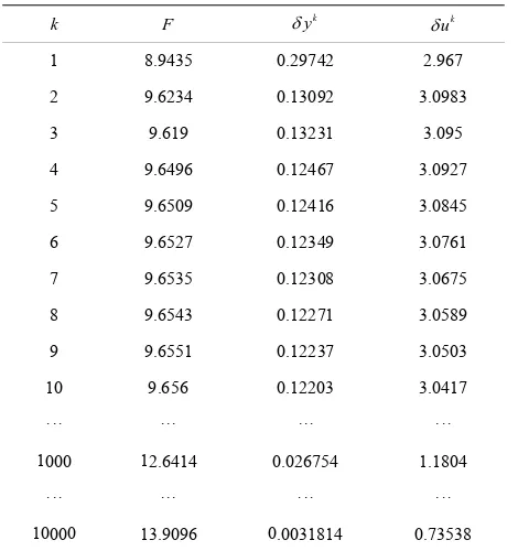
 . The smallest value 109 was reached tar d from s te 1.

In the tables below (Tables 1 and 2) is the number of an iteration,

k F

terat

is the value of th ective function on the current i ion,

e obj

2

k k

L

y y y

   and

2

k k

L

u  uu , the calculation results for the 100 100

 

are presented. We constructed the exact solution

 

y u,

of the discrete optimal control problem, so, we knew the exact minimum of the cost function F14.5293.

We can conclude that block SOR method had a big omp

ns w made for the different

st t

sh

advantage in c arison with preconditioned Uzawa method in the accuracy of the calculated state y and

con-trol u.

A number of calculatio ere

[image:5.595.307.538.97.361.2]

ate and control constrained optimal con rol problems on the different me es. All of them demonstrated the pref-

Table 1. Uzawa method.

k F k

y

 k

u 

1 8.9435 0.29742 2.967

2 9.6234 0.13092 3.0983

3 9.619 0.13231 3.095

4 9.6496 0.12467 3.0927

5 9.6509 0.12416 3.0845

6 9.6527 0.12349 3.0761

7 9.6535 0.12308 3.0675

8 3.0589

9.6551 0.1223 0503

1 1

10 0 0

9.6543 0.12271

9 7 3.

10 9.656 0.12203 3.0417

··· ··· ··· ···

000 2.6414 0.026754 1.1804

··· ··· ··· ···

[image:5.595.57.292.479.729.2]

00 13.9096 .0031814 0.73538

able 2. OR meth

F k

y

 k

u 

1 41.9339 4.5763 0.077971

2 3.9872 4. 5

36.4 3. 0.

4.227 3.7676 5.7309

31 3. 1

6 4.79 3.1618 5.6581

1.

8 5.6163 2.6164 5.5933

24.03 5 2.1819 1.6349

1 6.9 5

3 2.3

439 .8003

3 713 8831 51251

4

5 .6414 2552 .0026

7 27.5472 2.6887 3318

9 8

10 6.5528 2.1301 5.5033

··· ··· ··· ···

000 14.4687 224e−00 0.15564

··· ··· ··· ···

695 14.525 759e−006 0.0098418

eren f th e meth ed on the y of the state equat the com with the -tioned Uzawa ds, whil ere faster gent than e grad thods ap or the pro th the p alization e state c

REFERE

ES

[1] . Lio imal C stems Gouverhed by rtial Di ntial Equati , New York, 1971. doi:10.1007/978-3-642-65024-6

ce o e iterativ ion in

ods bas parison

penalt precondi metho e that w conver th ient me plied f blems wi

en of th onstraints (see [9,10]).

NC

J.-L ns, “Opt ontrol of Sy

Pa ffere ons,” Springer-Verlag

[2] eitta J. Spr Tiba, ion

of Elliptic Systems. Theory and Applications,” Springer-

for Finite-Dimensional Constrained Saddle Point Problems,” Lobachevskii J ol. 31, No. 4, 2010, pp. 309-322.

pany,

State University, Kazan, 2008.

rk, 1988.

P. N anmaki, ekels and D. “Optimizat Verlag, New York, 2006.

[3] P. H. Ciarlet and J.-L. Lions, “Handbook of Mumerical Analysis: Finite Element Methods,” North-Holland, Am- sterdam, 1991.

[4] A. Lapin, “Preconditioned Uzawa-Type Methods ournal of Mathematics, V

[5] R. Glowinski, J.-L. Lions and R. Tremolieres, “Numeral Analysis of Variational Inequalities,” Translated and Re-vised Edition, North-Holland Publishing Com

sterdam, New York and Oxford, 1981.

[6] A. Lapin, “Iterative Solution Methods for Mesh Varia- tional Inequalities,” Kazan

[7] I. Hlavacĕk, J. Haslinger, J. Necăs and J. Lovisĕk, “Solu- tion of Variational Inequalities in Mechanics,” Springer Verlag, New Yo

-462.

Sum of a Quadratic and a Convex Functional,” Izvestiya Vysshikh Uchebnykh Zavedenii. Matematika, No. 8, 1993, pp. 30-39.

[9] A. Lapin and M. Khasanov, “State-Constrained Optimal Control of an Elliptic Equation with Its Right-Hand Side Used as Control Function,” Lobachevskii Journal of Ma- thematics, Vol. 32, No. 4, 2011, pp. 453

doi:10.1134/S1995080211040287