Supply chain optimization using an incremental
approach: the improved WDScan model
I
Summary
Albert Heijn is a large supermarket chain in the Netherlands that supplies around 900 stores in the Netherlands from its four distribution centres across the Netherlands. Most of these stores are delivered on a daily basis for each flow of goods. The deliveries of the ambient and fresh goods are scheduled in delivery windows of one hour. In order to gain more insight in the total costs of a delivery time window plan (DTWP) Albert Heijn has developed a model with ORTEC: WDScan. However, this model does not give acceptable results. The DTWP WDScan creates is not acceptable, because (1) it does not imply lower overall costs than the manually generated DTWP and (2) the manual DTWP is considered infeasible by WDScan, while this DTWP is currently used and therefore feasible. Our goal is to improve the WDScan model to make sure that it can be used to generate feasible and improved delivery time window plans for the busy weeks. The busy weeks are chosen, because changing a DTWP in these weeks is accepted by the stakeholders, while in normal weeks it is not accepted to change the DTWP.
In literature, the DTWP problem is related to an Inventory Routing Problem (IRP). An IRP is a generalisation of the well-known vehicle routing problem (VRP), first introduced by Danzig and Ramser (1959) as the Truck Dispatching Problem. The problem most related to the DTWP problem is the periodic inventory routing problem introduced by Gaur and Fisher (2004). Gaur and Fisher (2004) introduce a method to cope with this problem at Albert Heijn. The difference between the periodic inventory routing problem and the DTWP problem is that Gaur and Fisher (2004) solved the actual truck routing while our problem mainly focusses on an estimation of the costs of transportation. In addition to the transportation costs, our problem considers the distribution centre and store costs. The DTWP problem also involves the importance of not bothering customers at the stores of Albert Heijn by restocking. Besides the difficulty of assessing the transportation, store, and distribution costs, the importance of not bothering customers by restocking should be taken into account.
In order to improve the WDScan model, we analyse the input and parts of the WDScan model. We identify three areas for improvement. The first area for improvement is the delivery size estimation. Currently, the values for the delivery size of a delivery to a store are fixed per day, based on historical data. Therefore, the delivery size is the same when the delivery time window is in the morning or in the evening. However, in practice the delivery size is based on the expected number of customers until the next delivery.
The second area for improvement considers the penalty functions used in WDScan. Our analysis shows that the penalty functions of WDScan need improvement. The main reason the penalty functions have to be improved is that they are a large portion of the target function, while this should not be the case for a feasible solution. In addition, the manual feasible DTWP yields a lot of penalty costs, while feasible solutions should not yield high penalty costs.
II are picked in advance. Order picking in advance allows solutions that are infeasible with just-in-time order picking.
We propose three solutions to improve the above mentioned areas for improvement. The first solution is a method to estimate the change in delivery size when changing a heartbeat moment. A heartbeat moment is the delivery time window throughout the week. When changing such a heartbeat moment, all of the delivery windows are set at the new heartbeat moment. Based on the amount of customers a delivery supplies, we calculate the amount of goods for each sales hour. When changing the heartbeat moment the amount of goods of the delivery is calculated by the sum of the goods for the hours until the next delivery. We show that this gives a good estimate of the delivery size when changing the heartbeat by testing the method for different stores with similar customer patterns, but different heartbeat windows.
The second solution is the improvement of the penalty functions of WDScan. We propose changing the penalty functions based on the guidelines by Smith and Coit (1997). Smith and Coit (1997) argue that penalty functions should be severe enough to penalize infeasible solutions, but not too high to not allow infeasible solutions that are close to the optimal region. We introduce upper bounds for the penalty functions that are severe enough to penalize infeasible solutions.
The third solution involves changing the just-in-time order picking model in WDScan. We propose to use a method that supports order picking in advance. This method is based on the method currently used by the SCCP department of Albert Heijn to assess whether the manual DTWP is executable in the distribution centres. The main assumption is that if the orders can be picked in advance by a shift of order pickers and does not surpass the maximum loading dock buffer area, a valid order picking plan can be created. Our method can determine the minimum costs and use of buffer capacity given the model assumptions.
III
Preface
This thesis is the final stage of my master Industrial Engineering and Management, track Production and Logistics Management. I worked with great pleasure over the last six months at Albert Heijn. I would like to thank the whole Supply Chain Capacity Planning department for the pleasant time working there. Especially, I would like to thank Adze Spoelstra and Martijn Beerepoot for their feedback, guidance and support. I would also like to thank Liesbeth Brederode and René Baks for giving me the opportunity to conduct this research project at Albert Heijn.
In addition to my supervisors at Albert Heijn, I would like to thank Marco Schutten and Leo van der Wegen for their feedback and counselling. You have made sure the level of this thesis has been greatly improved.
Finally, I would like to thank my friends and family for their unconditional support during my studies. You have given me the strength and courage to finish this project.
IV
Contents
Summary ... I Preface ... III Glossary ... VI
1. Introduction ... 1
1.1 Introduction to Albert Heijn and the SCCP Department ... 1
1.2 Problem definition ... 2
1.3 Research goal and sub questions ... 3
1.4 Outline... 4
2. Current situation and WDScan model ... 5
2.1 Manual process of determining the delivery time window plan ... 5
2.2 The ORTEC Solution: WDScan ... 9
2.3 Analysis of WDScan ... 13
2.4 Conclusion ... 22
3. Literature review ... 23
3.1 CO problems ... 23
3.2 Basic VRP ... 24
3.3 The inventory routing problem ... 26
3.4 Simulated annealing... 29
3.5 Penalty functions ... 30
3.6 Conclusion ... 32
4. The improved WDScan model ... 33
4.1 Improved delivery size estimation ... 33
4.2 Improved penalty costs model ... 38
4.3 Improved order picking model ... 44
4.4 Conclusion ... 51
5. Conclusions and future research ... 53
5.1 Conclusions ... 53
5.2 Recommendations ... 54
5.3 Future research ... 56
References ... 58
Appendices ... 60
Appendix A: List of input parameters ... 60
Appendix B: Cluster Analysis ... 61
V List of Figures
Figure 1: Order picking amount, adapted from Albert Heijn (2014) ... 6
Figure 2: Buffer usage, adapted from Albert Heijn (2014) ... 6
Figure 3: Current situation of determining DTWP for the busy weeks ... 8
Figure 4: WDScan connections ... 9
Figure 5: Distribution Centre process, adapted from ORTEC (2013) ... 10
Figure 6: Store process, adapted from ORTEC (2013) ... 11
Figure 7: Selection of items to improve ... 15
Figure 8: WDScan target function parts for the current DTWP ... 18
Figure 9: Penalty costs of the current DTWP ... 19
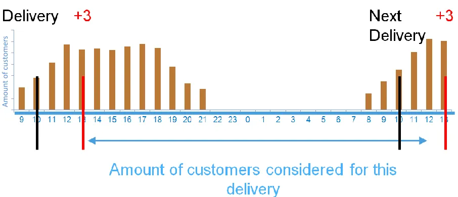
Figure 10: What customers are considered for a delivery in our model? ... 35
Figure 11: Calculation of packages per hour... 36
Figure 12: Target function value after a run of WDScan ... 40
Figure 13: Determining the upper bound of the store interval time penalty ... 43
Figure 14: Distribution Centre process, adapted from ORTEC (2013) ... 44
Figure 15: Order picking amounts in WDScan ... 45
Figure 16: WDScan order picking amount v actual order picking amount ... 46
Figure 17: Improvement order picking model, N being the number of order pickers ... 50
Figure 18: Model requirements WDScan for determining the DTWP for BWs ... 55
Figure 19: Customer pattern over the week for selected stores ... 61
Figure 20: Delivery size fractions over the days for selected stores ... 62
List of Tables Table 1: Different characteristics of Customers, Vehicles and Objective functions for the VRP (Toth & Vigo, 2002) ... 25
Table 2: Different solution techniques ... 29
Table 3: DTWP for the fresh goods of a single store ... 33
Table 4: Correlation between delivery sizes of stores, when selecting the same heartbeat moment ... 37
Table 5: Penalty overview for current DTWP... 39
Table 6: Comparison current DTWP to WDScan optimization ... 40
Table 7: New penalty functions ... 42
VI
Glossary
AH (Albert Heijn B.V., a subsidiary of Ahold N.V.): the company this research is conducted at.
BW (Busy Weeks): the busy weeks are for example the weeks before Christmas or Easter where a lot more goods have to be delivered to the stores.
Current DTWP: the manually constructed current DTWP. The current DTWP is often used in this research as a benchmark for the results of WDScan.
DC (Distribution Centre): one of the regional distribution centres of AH.
DTW (Delivery Time Window): the time window a delivery to a store for one of the flows (ambient or fresh) is made in. The DTWs of all of the stores of a distribution centre is called a Delivery Time Window Plan for this distribution centre.
DTWP (Delivery Time Window Plan): the plan of the delivery time windows for all of the stores connected to one distribution centre. This DTWP gives the delivery times for all of the stores and days of the week. The delivery time window is at the heartbeat moment, the same moment for every day. In addition, if we speak of a DTWP of a store we mean the part of the DTWP considering this single store.
Franchise: the term used to indicate that a store is not owned by Albert Heijn but rather is owned by an entrepreneur who is the franchisee of the Albert Heijn brand.
Heartbeat moment: the timeslot a store is delivered. This timeslot is the same every day of the week, if a delivery is made to this store on this day.
Infeasible DC Closed Loading: a penalty for each trip that leaves the Distribution Centre (DC) outside of the opening hours of the Distribution Centre loading time of the DC
Infeasible DC Closed Production: a penalty for each trip that has its order picking conducted outside of the order picking opening hours of the DC
Infeasible DC Prod Spread: a penalty per roll cage (RC) outside of the given bandwidth for a set amount of hours (parameter). The average over these hours is calculated and all the RCs outside of the given bandwidth result in a penalty per RC. The penalties are calculated for all of the flows, and the sum over all of the flows.
Infeasible DC Trip Departure: a penalty when less than a given threshold value or more than the capacity of the DC amount of trucks depart from the DC for all the hours a trip is made. The amount of trips can be a non-integer.
Infeasible Store Closed: a penalty for if the start restocking is after the store is closed. Per store a parameter for the time after closing restocking is allowed.
VII deliveries that are not of the same flow, two hours is required. Violating this restriction gives a penalty per minute violation.
Infeasible Truck Type Spread: a penalty per truck outside of the given bandwidth for a set amount of hours (parameter). The average over these hours is calculated and all the trucks outside of the given bandwidth result in a penalty per truck. The penalties are calculated for all of the truck types, and the sum over all of the trucks.
Infeasible Truck volume: a penalty for using more than the capacity of a truck per RC. Per RC over the truck capacity a penalty is inflicted.
RCs (Rolcontainers, Dutch): load carriers used in the process of transport of goods between the distribution centres and the stores.
WD (Winkeldistributie, Dutch): the project initiated to improve the delivery time window plan (DTWP) for the stores, distribution centres, transportation and customers in the store. One of the outcomes of this project is the WDScan model.
1
1.
Introduction
This chapter introduces the research project. This thesis is the final part of my master program in Industrial Engineering and Management, conducted at the Supply Chain Capacity Planning (SCCP) Department of Albert Heijn (AH), introduced in Section 1.1. In addition, Section 1.1 presents the motivation for the research. Section 1.2 gives the problem definition based on the initial problems as stated by Albert Heijn. Section 1.3 presents the research goal and the sub questions. This chapter finishes with the outline of this thesis in Section 1.4.
1.1
Introduction to Albert Heijn and the SCCP Department
Albert Heijn (AH) is a subsidiary of Ahold and is situated in the Netherlands. Its headquarters are located in Zaandam and it supplies around 900 stores in the Netherlands and a few stores in Belgium, from different distribution centres across the Netherlands. The deliveries are made on a daily basis and for different flows of products. An example of such a flow is the flow that contains the fresh (cooled) goods, which are delivered separately from the ambient goods.
The delivery time windows for the stores are based on past practice, and revised occasionally if for example a new store has to be added or a delivery time window of an existing store has to be modified. The creation and modification of the delivery time window plan (DTWP) is a lengthy process that involves a lot of communication with the store managers, the operational managers and the supply chain partners. If a change in such a window is approved, a process of trial and error in changing time slots has to result in a feasible solution. Albert Heijn would like to use a better solution and make the process of determining these new delivery windows less time consuming.
In the current situation these delivery times are used as input for the transportation department of Albert Heijn that creates the vehicle routes based on these delivery windows. Based on this transportation plan, the distribution centres create their capacity plan. This process is based on optimizing small parts of the total distribution chain. In order to get a better overall output, Albert Heijn would like to have the delivery windows determined based on costs in the stores, the amount of customers that are bothered by the restocking of the shelves in the stores, the costs in the distribution centres and the total transportation costs. Taking all of these criteria into account, Albert Heijnhopes to get a better overall performance.
2 The main problem as indicated by Albert Heijn is the bothering of customers when restocking the shelves during peak times in the stores. The goal is to reduce the amount of customers bothered by restocking, without implying additional costs in the total value chain. This includes the store, transportation and DC costs. The project “Winkeldistributie” (WD) has tried to facilitate this; however because of a lack of support from different departments among Albert Heijn this has not reached its potential. The future state desired by Albert Heijn is a centralised approach aimed at reducing overall costs, while creating additional value for their customers.
The problem WD has to solve is a typical multi-disciplinary problem, as it involves a lot of different actors. In this case the impact of a change in the delivery windows involves a lot of different departments of Albert Heijn. These departments all optimize their plan in a certain way. The project WD has tried to optimize1 the total value chain costs, instead of optimizing the costs for each department separately.
The assignment is to see how we can improve the delivery times created for these more busy weeks where changes are permitted. The current situation is that the DTWP is created ‘by hand’, building the DTWP from scratch in Excel. Albert Heijn wants to see if this can be improved by using WDScan to determine the delivery windows. However, the WDScan application is not creating acceptable delivery times yet, and a part of the solution is to make changes to the model. If there is a way to get these busy weeks improved, Albert Heijn likes to see how this can be used for the normal weeks. However, to assess how WDScan can be used for the normal weeks is outside the scope of this research.
1.2
Problem definition
This section describes the problem identification and analysis. Identifying the problem is done based on interviews with supply chain officers of the SCCP Department of Albert Heijn. The initial goal of project WD was to reduce the amount of customers bothered by restocking and optimizing the sum of transportation, DC and store costs. The DC costs are the sum of the costs of distribution centres of Albert Heijn in the Netherlands.
The problems as stated by Albert Heijn are (Beerepoot & Spoelstra, Interview 1, 2014):
Customers are bothered by restocking during customer peak time
It is not possible to gain insight in the total costs of a DTWP and customers bothered
The process of determining the delivery time window plan (DTWP) is a manual process
A lot of departments and stores (stakeholders) all have a say in the processThe main issue in having a manual process and the urge to reduce the amount of customers bothered by restocking, is evaluating what effect a change to the DTWP has. In order to reduce the amount of
1
3 customers bothered and total costs, we have to know what costs a change implies. In the current situation it is not known in advance what a change inflicts. In addition, the way the DTWP changes are evaluated should be accepted by all of the stakeholders that are affected by such a change.
As described in Section 1.1, Albert Heijn has tried to facilitate this with the project WD. However, this project finished without a proper implementation of a model to facilitate this for the SCCP department. This year a new project ‘WDScan’ was initiated to implement the model built during the project WD at the SCCP department. The main question posed by the SCCP department is:
‘How can WDScan be used to improve the delivery time window plan process?’
Section 1.3 rephrases this question to a research goal. The SCCP department thinks it is best to use WDScan for the busy weeks (BW), because they do not have to take all of the stakeholders into account when creating the DTWP for these weeks. We do not have to take all the stakeholders into account, because the stakeholders accept changes in the DTWP for the BWs. Contrary to the regular weeks, weeks where the stakeholders only accept minor changes to the DTWP. In addition, Section 1.3 explains what research questions we use to reach the research goal.
1.3
Research goal and sub questions
The research goal of this thesis, as explained in Section 1.2, is based on the question of the SCCP department to see how we can use WDScan to improve the DTWP process. At the SCCP department there is reasonable doubt about the outcomes of the model and they would like to gain more insight in how the model works and what parameters influence the outcome of the model most. The research goal is therefore:
“Provide a plan to use WDScan to make better decisions on store, distribution centre and transportation costs versus the amount of customers bothered for the busy weeks”
This research goal implies we improve the current situation into a more desired situation. To achieve this goal we have created several sub questions. In order to change the current situation to the desired situation, we have to investigate the current situation. Therefore our first research question is: ‘How are the time windows determined in the current situation?’ Once we know the current situation, we can find improvements to the current situation. Our second research question investigates the model built by ORTEC and its possible drawbacks and benefits. Therefore, our second research question is: ‘What does the WDScan method look like, and what are its benefits and drawbacks’
4 After assessing the WDScan model, we give suggestions to improve parts of the model. The suggestions are based on the literature review and interviews with experts of the SCCP department. As stated in Section 1.1, Albert Heijn wants to use the improved model for the busy weeks (BW). The reason to investigate the BWs is that the SCCP department thinks implementing WDScan for these weeks is easier, because in the BWs the stakeholders accept changes to the DTWP. For example, the store managers of Albert Heijn accept that their delivery times change in these weeks. However, in order to use the model for these weeks we have to assess if the method is able to cope with the busy weeks. The research question is therefore as follows. ‘How can we improve the WDScan model and what is the performance of the improved model?’
Summarised, we have formulated the following research questions: 1. How are the time windows determined in the current situation?
2. What does the WDScan method look like, and what are its benefits and drawbacks
3. What are similar problems to the WDScan problem in literature, and what are possible solutions for this problem in literature?
4. How can we improve the WDScan model and what is the performance of the improved model?
1.4
Outline
The research questions mentioned in Section 1.3 are the guidelines for the chapters in this thesis. Hence, the thesis first explains the problem and the background of the problem, and then continues to illustrate the current situation and the solution proposed by ORTEC. The following chapters analyse the WDScan model, suggest improvements and test these improvements. The final part of the thesis considers conclusions and future research.
Chapter 2 concentrates on explaining the current situation and the solution proposed by ORTEC: WDScan. By explaining the current situation and demonstrating how the WDScan model works we lay the base for the analysis of the WDScan model. This chapter illuminates several drawbacks and advantages of the WDScan model. In addition, this chapter selects items to improve to the WDScan model. Chapter 3 answers the third research question, by assessing what literature is available to tackle the problem WDScan tries to solve. To do this, we first have to classify this problem. This clarifies what solutions are readily available in literature and what the gaps are in the available literature. In addition, it presents literature on parts of WDScan that require further investigation.
Chapter 4 focusses on the improvements that we advise for the WDScan model. This chapter presents improvements to the ORTEC model based on the drawbacks of the model as explained in Chapter 2. The chapter continues by giving the validation of the improvements. Here, quantitative and qualitative validation shows why the improved methods should be implemented. In addition, additional steps that have to be taken by Albert Heijn to use the WDScan method for the busy weeks are presented.
5
2.
Current situation and WDScan model
This chapter answers the first two research questions: ‘How are the time windows determined in the current situation’ and ‘What does the WDScan method look like, and what are the benefits and drawbacks’. To answer these questions, Section 2.1 first illustrates the manual process of determining the delivery time window plan (DTWP) for the busy weeks (BW). It describes the process and gives a schematic overview of the process under investigation. Section 2.2 focusses WDScan, the solution proposed by ORTEC to solve this problem. This section is divided in the input, model choices and output of WDScan. Section 2.3 analyses WDScan and identifies what the advantages and drawbacks are of WDScan, and presents the selection of the parts of WDScan to improve. Finally, Section 2.3.3 gives the conclusions of this chapter.
2.1
Manual process of determining the delivery time window plan
To answer the first research question: ‘How are the time windows determined in the current situation?’,
this section explains the current manual process of determining the delivery time window plan (DTWP). This process is a manual process and starts 20 weeks before the busy weeks (BW). Based on the most recent DTWP of a regular week, indexed for the forecasted volume increase, a tactical plan is created. Based on the forecast and the regular DTWP, the supply chain specialists determine what plan should be used as a base for each of the days in the busy weeks. The amount of goods of these deliveries is adjusted for the volume increase expected by Albert Heijn for these days. Because the amount of goods that has to be delivered to the stores is higher than in a regular week, the regular allocation of trucks is not valid anymore. To assess whether more deliveries to a store are necessary, the amount of load carriers (RCs) for a delivery to a store is compared to the RC capacity of a truck. If the amount of RCs plus a safety margin is larger than the truck capacity, an additional delivery to the store is scheduled. Additional deliveries are scheduled, because the truck scheduling algorithm, Shortrec, does not generate additional deliveries. The truck scheduling algorithm solves a Vehicle Routing Problem (VRP) with time windows (Sections 3.2. and 3.3 explain the VRP in more detail).
The additional delivery to a store is preferably placed on the heartbeat moment of this store, a time window equal to the delivery rhythm of this store throughout the week.If the first step is completed for all of the deliveries to all of the stores, the next step is initiated. This next step is called ‘simulation’; here a rough transportation plan based on the DTWP is created. The transportation plan shows the routes of the trucks and what stores are combined in a truck. In addition, this transportation plan visualises how many trucks have to leave the Distribution Centre (DC) each fifteen minutes. Based on the amount of trucks that leave the DC each fifteen minutes, the SCCP department determines whether the DTWP is ‘executable’ for the four DCs. The following points are evaluated, and explained in more detail in the remainder of this section:
6 Is the percentage of goods that has to be picked at night below a certain (predetermined)
threshold value?
[image:14.612.73.541.248.363.2]Based on the above mentioned points the DTWP is evaluated. If one of these restrictions is not met, the SCCP department is requested to make changes to the DTWP. Typical changes are moves of a certain amount of volume to the previous or next hour. Based on these requests a number of delivery time windows are rescheduled. Figure 1 illustrates how changing these time windows can help to ensure that the amount that has to be loaded is within the maximum capacity. The dashed line in Figure 1 shows the order picking amounts per hour that had to be picked before changing the DTWP. The dotted line shows the amount that has to be picked after the changes have been made. Where the dashed line surpasses the solid capacity line more than once, the dotted line is completely below the maximum capacity line.
Figure 1: Order picking amount, adapted from Albert Heijn (2014)
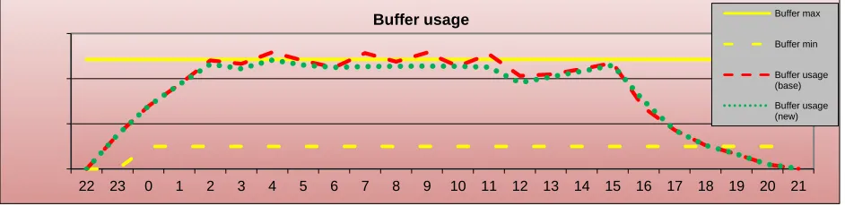
[image:14.612.72.543.501.616.2]In addition to the order picking amount, the usage of the buffer area has to be below the capacity threshold. The buffer area is the area where the RCs are waiting before they are loaded into the trucks. In front of each loading area there is a buffer area that can buffer at most two truckloads. Figure 2 illustrates the total buffer usage, before the changes to the DTWP and after the changes. The dashed line, the buffer usage of the base DTWP, surpasses the maximum of the buffer several times. While the dotted line, the buffer usage of the new DTWP, never surpasses the maximum buffer capacity line.
Figure 2: Buffer usage, adapted from Albert Heijn (2014)
Figures 1 and 2 are based on the transportation plan created from the DTWP. This transportation plan is created using Shortrec, a software package supplied by ORTEC. Based on the departure times of trips from the DCs of Albert Heijn the amount of goods that has to be loaded is calculated. The dotted green
22 23 0 1 2 3 4 5 6 7 8 9 10 11 12 13 14 15 16 17 18 19 20 21
Amount of goods that have to be loaded Order picking capacity
Start loading amount (base)
Start loading amount (new)
22 23 0 1 2 3 4 5 6 7 8 9 10 11 12 13 14 15 16 17 18 19 20 21
Buffer usage Buffer max
Buffer min
7 lines in Figure 1 and 2 show the improved DTWP, while the red dashed line shows the starting point of the improvement. After changing the delivery times of different stores, another rough transport plan is generated. Because the transport algorithm only does two iterations, while it would do at least twelve to create the final plan, the result is called a rough transportation plan. The reason for doing another iteration is that the route planning algorithm has different delivery time windows for a significant amount of stores. Different delivery time windows could result in a different amount of goods that has to be picked compared to the first plan. In addition, doing a second run is a check to see if the changes that are requested by the DCs are honoured and to filter possible errors made in the manual process. Doing more than two runs would not increase the performance substantially, because most of the issues are resolved after one run (Beerepoot & Spoelstra, Interview 1, 2014). This process is done for all of the days that have a high volume (as indicated in the tactical plan), for all of the DCs. The process of building the DTWP, running all of the individual high volume days with Shortrec for all distribution four distribution centres, updating the DTWP and run the new DTWP in Shortrec takes two fulltime weeks of four employees for the busy weeks around Easter.
8 20 Weeks before
the BW that have to be planned
Tactical plan
Apply tactical plan to base schedule
Make deliveries fit in truck
Simulation
Allowed schedule?
Use the improved time windows
Yes No
Tactical plan
Determine the base DTWP per day and volume increase per day
Determine the amount of RCs For all deliveries
For all days
Simulation
Create rough transport and order picking plan
for DC
Set delivery window to the requested new
window Able to change delivery window?
Yes
For all DCs
Make deliveries fit in truck
Amount of RCs > capacity truck? Yes
Check next delivery
No For all stores and
deliveries
All deliveries done Heartbeat
delivery possible? Find another time
window No
Does the proposed moment interfere with
another delivery?
Yes
Yes
Update RC numbers for the added and original
delivery No
Use heartbeat moment Add a delivery for
this store Requests per hour to move volume to another time slot
Request delivery availablity of stores Request fulfilled? More changes available?
Go to next hour
No Go to next delivery
Yes
Yes No
No All hours done
All deliveries done
All days done Go to next day
All DCs Done
[image:16.612.115.546.70.627.2]End
9
2.2
The ORTEC Solution: WDScan
To answer the first part of the second research question ‘What does the WDScan method look like and what are its advantages and drawbacks’, this section provides insight in the WDScan model built by ORTEC and its advantages. This section gives a general impression of the model. Section 2.3 provides a more in depth view of the model and displays its drawbacks by giving a thorough analysis of the model. Section 2.2.1 gives an overview of WDScan and its advantages. Section 2.2.2 describes the input part of WDScan. Section 2.2.3 explains the WDScan model. Section 2.2.3 elaborates on the output of WDScan.
2.2.1 The purpose and advantages of WDScan
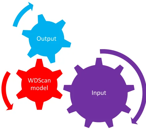
[image:17.612.137.373.348.560.2]The WDScan model was built to improve a more general situation of the process described in Section 2.1. It was built to determine what the best DTWP in general is, when taking into account store, DC and transportation costs and the amount of customers bothered; the problem as described in Section 1.2. However, the DTWP that WDScan creates is not acceptable, because (1) it does not imply lower overall costs than the manually generated DTWP and (2) the manual DTWP is considered infeasible by WDScan, while this DTWP is currently used and therefore feasible. In order to gain insight in the model it is important to know how the parts are connected. Figure 4 gives an idea how the different parts of WDScan are connected.
Figure 4: WDScan connections
As seen in Figure 4 the input gear is relatively large; this represents the importance of the input. In the WDScan model, input is not just raw data. In addition to raw data, output of other models is used. An example of such output is the output of a congestion model. However, some of these input parameters are based on simple assumptions. Based on this input data, WDScan evaluates the costs of a certain DTWP. The WDScan model calculates the costs and customers bothered, and uses simulated annealing to improve this costs function incrementally.
Input WDScan
10 2.2.2 The input of WDScan
The input has a major influence on the results of WDScan. A lot of data is used in the model to calculate the costs of a certain DTWP, for example for every store the amount of customers for each hour of each day. In addition, there are some generic input data entries, for example the transportation costs per km and transportation costs per hour. These parameters do not change over time or when driving to store X instead of Y. However, they can be changed for the different kind of vehicles that are available to Albert Heijn. Based on the characteristics of a distribution centre (DC) input parameters vary, for example the order picking costs for each hour, DC, day and flow (ambient or fresh goods).
The amount of goods that has to be delivered to the stores and the amount of customers are input data. The value of these input parameters is determined for each store, day, hour and flow. Several input parameters are based on choices rather than on raw data. In addition, for some input parameters store specific values could be defined, but rather a general value is used. This creates a lot of freedom, because we can change the output of the model by modifying input data. Increasing the level of detail of these parameters changes the output significantly.
2.2.3 The model choices of WDScan
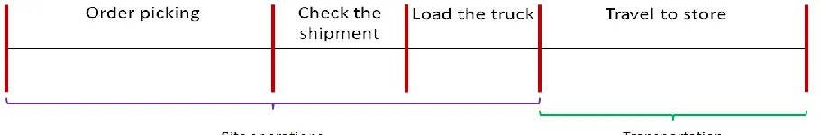
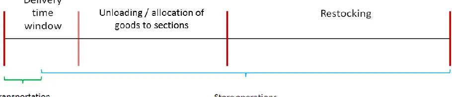
[image:18.612.82.537.508.583.2]One of the key assumptions of the WDScan model is that the flow of a delivery is as shown in Figure 5 and Figure 6. WDScan assumes that all these activities are direct predecessors and are started when the former is completed. Figure 5 shows the process at one of the DCs (distribution centres) of Albert Heijn. Based on the delivery time window chosen, the loading of the truck at the DC is finished at the beginning of the delivery time window, minus the time to travel to the store. The activities are therefore considered to be direct predecessors of each other, and calculated from the decision variable: the delivery time window of a single store. Figure 6 shows the store process, where the same assumptions are made as for the DC process: all activities are direct predecessors of each other. Here the unloading and allocation of goods to sections starts in the middle of the determined delivery time. The restocking starts when the unloading and allocation of goods to sections is finished.
11
Figure 6: Store process, adapted from ORTEC (2013)
All of the operations mentioned in Figure 5 and Figure 6 incline certain costs. The WDScan model calculates these costs for all of the stores and sums over all of the stores. In addition to the store, distribution centre and transportation costs, the amount of customers bothered is taken into account. The amount of customers bothered is the sum of the amount of customers bothered for each delivery made to store . To be able to compare the amount of customers bothered among stores, a method is created to compare this among different stores. Based on the model used by Albert Heijn to calculate the amount of customers bothered, ORTEC (2013) has formulated the following equation to calculate the customer bothered part of the target function:
∑
where each is a delivery and the customers bothered for a store is the sum over the customers bothered of all of the deliveries to store . The customers bothered is a part of the target function. The real costs in the target function are the distribution centre, store and transportation costs. In addition to these costs, penalty costs are present in the target function. Penalty costs occur if one or more restrictions are violated. However, these penalty costs increase the solution space for simulated annealing, and allow it to find more neighbour solutions. These penalty costs are also introduced, because the current DTWP used by Albert Heijn would not show a feasible solution in WDScan, because multiple restrictions are harmed in the current DTWP. Combining these components gives the following target function (ORTEC, 2013):
∑ ( ) ( ) ( )
( )
12 The store costs are calculated based on the amount of load carriers (RCs) delivered, and the time of the delivery. Per store, the input data states a costs value for restocking at a certain hour. These costs are multiplied by the amount of RCs delivered to the store at the delivery time window and divided by the restocking rate per store. In the WDScan input the restocking parameters are generic, not differentiated per store or hour.
The transportation costs are estimated by an model constructed by ORTEC that starts by selecting stores that could be delivered in one trip. It evaluates the costs of transportation using the delivery times of stores that are in the same cluster. The WDScan model creates clusters the following way (ORTEC, 2013):
Create a number of base stores that are the start of a cluster
Create a list of stores that are within a certain range of a base store that have the same DC and the same truck type
Clusters of stores can only be created between stores within this list
Based on a delivery time difference of less than 60 minutes, WDScan selects stores until the capacity of the truck is reached or the maximum number of stores in a cluster is reached.
If there are no more combinations to be made the remaining stores are delivered in a separate trip
The transportation costs are the sum of the time a trip takes, times the costs of a driver per hour and the km of a trip, times the costs per km. The transportation costs are allocated to the store that is delivered by this trip. If two or more stores are delivered in one trip, the costs are divided using a formula designed by ORTEC.
Finally, the DC costs are based on the time the orders have to be picked, loaded and unloaded. These tasks have certain fixed and variable amount of time. The different times are multiplied by the DC costs for the hours of the order picking and loading at the distribution centre. The distribution centre costs are allocated to individual stores. The costs in the distribution for order picking, checking the shipment and loading the truck for a delivery are allocated to the delivered store. If two or more stores are delivered in one trip, the formula used to divide the transportation costs is used.
2.2.4 Output of WDScan
The purpose of WDScan is to provide a better DTWP. Hence, the main output of WDScan is a new DTWP. In addition, WDScan provides performance indicators to analyse the solution. The output is written to an Excel file for convenience. This Excel file consists of:
A worksheet containing the new delivery windows of all of the stores for each flow (ambient and fresh). The amount of load carriers and goods (size of the delivery) are displayed for all of the delivery windows. The new DTWP is the output of the decision variable.
13 per store are shown for each store. The sum of these costs is the total costs associated with the DTWP2.
A worksheet containing the calculated time intervals for the total delivery. This worksheet states the time for every delivery: order picking starting time, the loading at the distribution centre start time and the time all of the other activities displayed in Figure 5 and Figure 6 start. Worksheets containing the amount of trucks in use, the amount of order picking at the DC and
the amount of outgoing trucks at the DC. These tabs give insight in the calculation of the global penalty costs. These penalty costs are explained in more detail in Section 2.3.3.
A worksheet containing the original DTWP, which is used as the start of the optimization process WDScan performs.
Worksheets containing the overview of the optimization process, displaying the objective value in the stages of the simulated annealing process. In addition, the parameter settings and penalty costs functions weights are displayed.
The output gives a good overview of how the model works and helps understand how the specific model choices actually work. A large part of the analysis is done modifying or structuring the output data to gain insight in the model. The analysis is explained in Section 2.3.
2.3
Analysis of WDScan
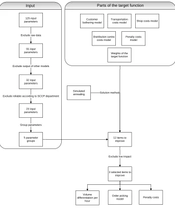
This section provides a more in depth view of the WDScan model. In order to answer the second research question: ‘What does the WDScan method look like and what are its advantages and drawbacks’, Section 2.2 introduced the WDScan model. This section elaborates more on the model and provides an analysis of the model to show the major drawbacks to improve. This section starts by explaining the approach used to analyse the model and then gives the outcome of the analysis. We choose this approach to better structure the analysis. The remainder of this section describes the analysis per group as described in the section containing the approach, Section 2.3.1.
2.3.1 Approach
In order to analyse the WDScan model we use several techniques: Interviews with the supply chain officers at the SCCP department, analysis of the output of WDScan, an in-depth analysis of the input variables and a quantitative analysis of the model choices in WDScan. In general we can split the non output part of WDScan model into input data and model choices, as explained in Section 2.2. We therefore use the same split in the analysis of the model. The approach used to analyse the validity of the model is to validate the individual input and model choices, in order to find flaws. To find flaws we investigate the output and investigate what causes the not expected output. Once the individual parts are validated or improved, the output should be re-validated to see if the improvements to the individual parts have resulted in improved output. The re-validation of the output is outside of the scope
2
14 of this thesis, because the improvements to the model first have to be implemented in order to test the output again.
Figure 7 schematically shows the approach used and outcome of the analysis. Based on the input parameters and the parts of the WDScan model, we have reduced the possible improvements to three groups to improve. Because there are a lot of input parameters, we reduce them to a few items that are interesting to improve. Based on interviews with supply chain officers and the analysis of the output we have reduced the huge list to 5 groups of items as possible improvements. Appendix A displays the list, containing the starting input data and considerations for improvement. We choose to exclude this from the body of the thesis due to the size of this list. However, this list is important, because it illustrates the process of selecting what input to consider neatly. Section 2.3.2 describes the analysis of the input part of the model. Here we describe in more detail the selection of the 5 groups of parameters. In addition we assess what of these parameters’ improvements are within the scope of the research and have a big impact on the outcome of WDScan.
In addition to the input, the model parts and solution method is investigated. The model parts are the parts of the target function:
The customer bothering model The transportation costs model The distribution centre costs model The store costs model
The penalty costs model
15 32 input
parameters 125 input parameters
55 input parameters
Input
Exclude raw data
Exclude output of other models
23 input parameters
5 parameter groups Group parameters
12 items to improve
Exclude low impact
3 selected items to improve
Penalty costs Order picking
model Volume
differentiation per hour
Transportation costs model Customer
bothering model
Simulated annealing
Parts of the target function
Distribution centre costs model
Weights of the target function
Penalty costs model
Shop costs model
[image:23.612.75.418.72.492.2]Solution method Exclude reliable according to SCCP department
Figure 7: Selection of items to improve
2.3.2 Motivation for what input items to improve
16 from a database with raw data for improvement. Examples of raw data are the average amount of customers for each hour for a specific store. These values are extracted from a database and put (almost directly) into the input file for WDScan. Another example of raw data is the address information of each store. The amount of input parameters that we start with is 125.
In order to find parameters that are interesting to improve, we excluded from investigation all of the raw data as possible subjects to investigate. However, the data in the databases has to be correct. Because the data subtracted from these databases is not modified and based on historical or location data, the SCCP department thinks most of this data is reliable. We do not investigate the raw data, except for the data Albert Heijn thinks is unreliable (Beerepoot & Spoelstra, 2014). This selection of input data results in 55 parameters remaining to investigate. The output data of other systems, if used as input for other planning systems at Albert Heijn is reliable for WDScan. Using the input used for other planning systems of Albert Heijn is reliable, because based on these models the costs for Albert Heijn are evaluated. An example of such output is the output of the congestion matrix, which is used in the normal transport planning process. The data that are not used in the normal planning process, or Albert Heijn thinks is not reliable, we include for investigation. 32 parameters remain after this selection. The remainder of the input data is specifically created for WDScan. In general these are based on practice, to model the current situation. Examples of this data are the restocking costs per hour. Parameters used to mimic decisions made in the current process are excluded from investigation. We keep the parameters that the SCCP department does not think are properly used on the list. The input rules are compared with the business rules used in the current (manual) process. The parameters that mimic the business rules of Albert Heijn properly are excluded. The 23 remaining parameters we group into five categories, which will be explained in the remainder of this section:
Costs of transportation, distribution centre and store per hour Time between two deliveries to a store
Amount of outgoing trucks per hour per DC per flow (ambient or fresh) Delivery size estimation between deliveries to a store
Delivery size estimation per hour
The remainder of this section argues whether or not to improve these groups of parameters. In the order of the above list we motivate what groups to improve. The selection is based on the impact of an improvement to one of these groups, and whether it is within the scope of this thesis to improve the group.
17 are verified, larger changes should be evaluated. The validation of costs changes is not within the scope of the project, because it is not possible to assess these costs changes within the time available to do this thesis.
The time between two deliveries to a store problem is solved when the penalty costs are properly assigned3. The time between two deliveries to a store is a restriction that we do not want to violate, except if there is no other possibility. Changing the penalty costs makes sure no restrictions are violated except if there is no other option. The time between two deliveries to a store restriction could be violated if a store has a very small delivery window or a lot of deliveries every day. The time between two deliveries to a store can be given per store, therefore changing this variable for the stores that have to violate the restriction solves the problem. Therefore, we solve this issue when improving the penalty costs.
The amount of outgoing trucks per hour per DC per flow is an input parameter to model the capacity restriction of the amount of trucks that can leave the distribution centre per hour. This parameter is correct in the current way of modelling the order picking process. However, because the SCCP department thinks the order picking model is not valid this parameter should be re-evaluated after improving the order picking model. Because we improve the order picking model4, we should re-evaluate this parameter.
The delivery size estimation between deliveries to a store is not investigated. A project to improve this estimation is done simultaneously to this thesis. The outcome of this project should be used to improve the model, however improving this estimation not within our scope.
Delivery size estimation per hour is chosen for improvement. The delivery size estimation per hour is the change in volume delivered to a store when changing a heartbeat moment. A heartbeat moment is the delivery time for each flow, where this delivery time is the same for every day a store is delivered for this flow. The volume changes are not that big when changing a heartbeat moment, however, they are an estimate of what amount of goods a store will receive. In order to gain the support of the stores that get changes in their heartbeat moment, it is important that the estimate is accurate. The store managers create a personnel schedule based on these estimates, and prefer an accurate estimation. The model proposed in Section 4.1 is accurate in predicting the amount of goods a delivery has when the heartbeat moment changes. WDScan currently uses a fixed amount of goods that does not change when changing a heartbeat moment, which is a good estimate for the ambient goods. However, for the fresh goods this can vary. In order to get a more accurate estimate of the delivery size, this has to be improved.
3
Section 2.3.3 explains the motivation for improving the penalty costs.
18 To conclude, we summarize the three input parameters that are selected for improvement. The delivery size estimation per hour is selected for improvement. The second input parameter we select for improvement is the amount of outgoing trucks per hour per DC per flow. The final input parameter selected for improvement is the time between two deliveries to a store. We note that merely the first selected improvement is stand alone, the latter two are both improved when improving parts of the model. The selection of the model choices to improve is described in Section 2.3.3.
2.3.3 Motivation of the model parts to improve
This section describes the motivation of what model parts to improve. We first explain the target function in detail and analyse the output of WDScan for a current delivery time window plan of Albert Heijn. The second part of this section explains what parts of the model we improve.
The target function of WDScan compares the real costs to the artificial costs. The real costs are the transportation, distribution centre and store costs. The artificial costs are the customers bothered (times a value for the customers bothered) and the penalty costs, as seen in the target function:
∑ ( ) ( ) ( )
( )
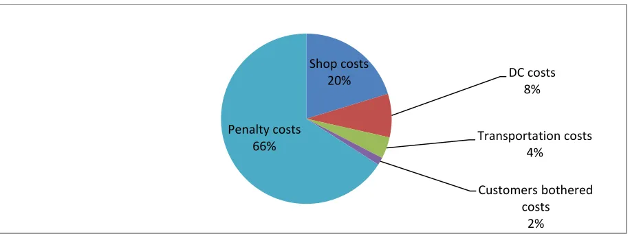
[image:26.612.82.540.491.663.2]The parameters , , and are used to display the relative importance of costs of different departments or costs of bothering customers. Balancing the real costs and the artificial costs is difficult, because in the penalty costs, some costs are implicitly modelled. For example, the truck spread penalty is used, because the transportation department wants to offer long journeys to the logistic service providers to get a better price per km. In order to get longer journeys, the amount of trucks should be evenly spread over the day, therefore a penalty is implied when the amount of trucks is not evenly spread. Figure 8 shows the contribution of the different parts of the target function to the objective value for a current delivery time window plan of Albert Heijn calculated by WDScan.
Figure 8: WDScan target function parts for the current DTWP
Shop costs
20% DC costs
8%
Transportation costs 4%
Customers bothered costs
2% Penalty costs
19 Figure 8 shows that the majority of the target function are penalty costs. The parameters and the penalty costs are the key to get good output of WDScan. The preference of Albert Heijn should be displayed in the parameters. However, to be able compare the real costs and customers bothered, the penalty costs should not be such a large part of the target function for a feasible schedule.
Based on interviews and analysis of the output, as described in this section, we motivate what parts of the model should be improved. The parts of the WDScan model are: the customer bothering model, the transportation costs model, the store costs model, the distribution centre costs model and the penalty costs model. In addition we investigate the weights of the target function and the use of simulated annealing. We analyse the parts of the model by getting an in depth view of the output of the model and how these costs are constructed. We first explain the parts of the model we select for improvement: the penalty costs model and the distribution centre costs model. We continue with explaining why we did not the select the other parts of the model for improvement.
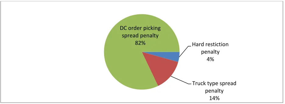
[image:27.612.71.539.504.675.2]We select the penalty costs model for improvement. The penalty costs are divided in different aspects: penalties for violation hard restrictions and penalties for violating soft restrictions. The hard restrictions are the restrictions we do not want to violate, except if there are no other options. An example is that Albert Heijn wants to have at least 2 hours between two deliveries to a store. However, some stores can only be delivered three hours a day and receive three deliveries. In this case it is not possible to have two hours between deliveries. In addition to the hard restrictions, soft restrictions are modelled in WDScan. The truck spread mentioned earlier in this section is one of the soft restrictions, the other one is the order picking spread. These restrictions have to make sure the truck usage or DC order picking amounts do not fluctuate too much over the days. Figure 9 shows the costs of the three different kinds of penalties: the order picking spread penalty, the truck spread penalty and the penalties for violating the hard restrictions. This figure shows that the majority of the penalty costs are order picking spread penalty costs and that the hard restriction violation penalty costs are just a small part of the costsin the current DTWP. The violation of hard restrictions is mostly due to restrictions that have to be violated, such as the time between two deliveries to a store, as mentioned earlier.
Figure 9: Penalty costs of the current DTWP
Hard restiction penalty
4%
Truck type spread penalty
14% DC order picking
20 The penalty costs model needs improvement. We divide the penalty costs model in the hard penalty costs and the soft penalty costs. We improve the hard penalties, because WDScan violates hard restrictions in favour of soft restrictions when improving the target function in the current penalty settings. This means WDScan moves from the feasible area when optimizing. We think the DC order picking spread penalty should also be improved, because it is such a large penalty in the current DTWP. We improve this penalty while improving the whole distribution costs model.
Improving the distribution centre costs model and its penalty costs is required, because a lot of penalties occur for the penalty related to the distribution centre costs model. The related penalty to the distribution centre costs model costs constitutes a large part of the penalty costs, as seen in Figure 9. Based on the output of the analysis we find that the order picking model, which is the main part of the
distribution centre costs model, is very different to the order picking model in practice. The order picking model in WDScan is based on just-in-time order picking, while the distribution centres of Albert Heijn order pick in advance. Therefore, the distribution centre costs model is selected for improvement by improving the order picking model.
We do not select the customer bothering model for improvement, because the model is similar to the current evaluation method of customer costs. The current method is based on whether the amount of customers is above the average amount of customers per m2 over all of the stores of Albert Heijn. If the amount is higher than the average amount plus a given amount, the amount of transactions per m2 is considered too high to restock at this moment. The model ORTEC built to measure the customer different; they count every customer during the restocking process as a customer being bothered. However, they square the amount of customers per m2. This means a larger amount of customers compared to the square meters is considered less favourable. This method is similar, however not the same. The fixed values in the original model pose another problem: they have to be indexed. The average amount of customers per m2 is used in the current model, based on the average over a certain period of time. The model used by ORTEC is robust to changes in the amount of transactions per m2,
21 We do not select the transportation costs model for improvement. The model used by Albert Heijn to create the transportation plan is built by ORTEC, the manufacturer of WDScan, therefore it seems reasonable to assume they share the same principles. After requesting more information about the model at ORTEC to investigate this, the consultant at ORTEC replied that the model used is ‘based on their own method, that has proven to be sound over a long time’ (ORTEC, 2014). This means we cannot get a measure from ORTEC about the accuracy of the heuristic, compared to the actual planning method. However, the transportation planners have validated that the output of this model seems reasonable in a previous version of WDScan. We do think the transportation model should be validated properly by comparing the output of WDScan to the output of the transportation algorithm used by Albert Heijn. We do not investigate this further, because Albert Heijn does not think the transportation model is flawed (Beerepoot & Spoelstra, Flaws in inputdata, 2014) . In addition, the impact on the target function is not as big as the other improvements, therefore we put this outside of the scope of this research.
We do not select the store costs model for improvement. The main reason for not improving the store costs model is that this is not yet applicable, because the penalty costs and order picking model are not valid yet. Changes to the store costs model will not have a large impact on the solution and target function value. We therefore suggest investigating this after improving the order picking model and
penalty costs model.
The use of simulated annealing5 is a good way to get to a better solution to our problem. Because a
large part of the WDScan target function is based on penalty costs in the current situation, simulated annealing can help to get out of a local optimum (ORTEC, 2013). Schutten (2013) claims an implementation of simulated annealing in practice requires a well chosen problem representation, an incremental costs calculation and a proper cooling schedule. We think the problem representation is usable for simulated annealing, because we can compare different costs. However, some of our costs are not actual costs. The choice of penalty costs and parameters should represent the preferences of Albert Heijn. This means the problem definition is a bit unclear at the moment, and should be improved. However, as explained in Section 2.3.3, this can only be done after the other improvements of Section 2.3.3. WDScan provides an incremental costs calculation, because neighbour solutions are created by changing a delivery time window of a store and evaluated on costs. However, in general, simulated annealing starts from a random initial solution (Henderson et al., 2003), while WDScan starts from the current DTWP. In addition, WDScan facilitates to lock some delivery time windows, because it is not accepted by Albert Heijn that these windows change. If a random initial solution is used, the locking of certain delivery time windows could not be facilitated.
We do not select the weights of the target function for improvement, because it is not yet applicable. This involves the weights of the parameters described in the start of this section. This has no use when
22 the penalty costs and order picking model is not valid yet. In addition, the soft penalty costs are closely related to this part, because they are not direct costs and should represent what direction the model should take. We therefore split the penalty costs into the hard restrictions and the soft restrictions. The soft restrictions should be taken into account when comparing the costs and customers bothered. To conclude, we summarize the model choices selected for improvement: the distribution costs model
and the penalty costs model. Where the hard penalty costs are improved and the soft penalty costs are not, because the soft penalty costs have to be evaluated when assessing the weights in the target function. However, we do improve one of the soft penalties: the order picking spread penalty, which is closely related to the distribution costs model. Assessing the weights of the target function and the customers bothered model are not within the scope of the research. The customer costs model is not selected for improvement, because the model is similar to the customer costs calculation in the current situation. The transportation model is not selected, because it was validated previously. We think
simulated annealing is a proper solution method for WDScan, mainly because of the use of penalty costs in WDScan.
2.4
Conclusion
23
3.
Literature review
The goal of this chapter is to answer the third research question: ‘What are similar problems to the WDScan problem in literature, and what are possible solutions for this problem in literature?’. To illustrate what similar problems are, we present the base problem, and show what kind of special case our problem is. Section 3.1 explains the general combinatorial optimization (CO) problem. Section 3.2 presents an example of a CO problem: the vehicle routing problem (VRP). Section 3.3 shows that our problem is comparable to an inventory routing problem (IRP), a general case of the VRP. In addition, this section explains the general IRP and in particular an implementation of an IRP at Albert Heijn from literature. Section 3.4 focusses on solving a CO problem and presents the simulated annealing method, used by WDScan. Section 3.6 describes methods to compare costs and qualitative matters. Section 3.5 gives insight how to cope with penalty costs. Finally, Section 3.6 states the conclusions of this chapter.
3.1
CO problems
A Combinatorial Optimization (CO) problem is a problem of finding an optimal solution among a finite number of possible solutions (Papadimitriou & Steiglitz, 1982). In combinatorial optimization a criterion
is measured by an objective, the objective is to maximize or minimize. Based on the decision variables a best alternative is chosen. The solution space covers all the possible solutions that are allowed by the
constraints and parameters. There are many fields in which CO has improved performance. In logistics examples of these fields are (Schutten, 2012):
Transport and Distribution Technical aspects of production Production planning and scheduling Allocation and location problems Warehousing
Healthcare
Among these CO problems, the Travelling Salesman Problem (TSP) is probably the most well-known (Aarts & Korst, 1989). The TSP a problem where a salesman has to visit certain cities exactly once in a tour, starting and ending at his home city. The objective is to minimize the total tour length. The travelling salesman problem is a nice example, because it is simple to explain and find a feasible solution to the problem, but finding the best solution is very difficult (Garfinkel, 1985). In a CO problem we minimize or maximize an objective, specified by a set of problem instances. These instances can be formalized as a pair ( ). The solution space S denotes the finite set of all possible solutions, and the costs function is defined as (Aarts & Korst, 1989):
24 In the case of maximization, satisfies
( ) ( )
Such a solution is called a ‘globally- optimal solution’ In this formulation ( )gives the optimal costs and the set of optimal solutions. The possible solutions are bound to constraints as mentioned before.
In general CO problems can be divided in two different classes: hard and easy problems. The difference between these problems is that the easy problems can be solved in polynomial time and of most hard problems it is not yet shown that they can be solved in polynomial time. Polynomial time means that if the problem gets larger, (and therefore computation time increases), the computation time will increase polynomially with the problem size. An example of an easy problem is an LP-problem. However, most problems that require variables to be integer are harder than non-integer problems (Vanderbei, 2008). Most real word problems require variables to be integer. For example, one cannot hire half an employee.
Most practical and theoretical problems are NP-hard. NP-hard problems cannot be solved in polynomial time and therefore a trade-off has to be made between optimality at immense computation time and sub optimality in polynomial time (Aarts & Korst, 1989). Due to the fact that easy problems are solvable in polynomial time and most practical problems are NP-hard, Section 3.4 dives into the different methods to ‘solve’ NP-hard problems.
3.2
Basic VRP
Since the first paper on the Truck dispatching problem (Danzig & Ramser, 1959) there have been a lot of papers on the Vehicle Routing Problem. A Google scholar search gives over 150,000 results for the term ‘Vehicle Routing Problem’. The problem that Danzig and Ramser (1959) describe is delivering gasoline to gas stations and they gave the first formulation of what we now call the VRP. Most papers are about how to solve the VRP or a problem closely linked to the VRP. The interest in the VRP is mostly because of its application in practice and the difficulty of the problem: the most efficient algorithms can solve VRP up to about 50 customers to optimality; some particular cases can be solved for bigger problem instances (Toth & Vigo, 2002)