Bachelor Thesis
The Boundary Layer over a Flat Plate
July 4, 2014
M.P.J. Sanders
Faculty of Engineering Technology Engineering Fluid Dynamics
Examination committee:
Prof.dr.ir. H.W.M. Hoeijmakers (Mentor/Chairman) Dr. H.K. Hemmes (External Member)
I Abstract
The properties of the boundary-layer over a flat plate have been investigated analytically, experi-mentally and numerically employing XFOIL. With the theory from Blasius and von K´arm´an, the boundary-layer properties over an infinitesimally thin flat plate have been investigated analytically. A finite thickness plate, designed to behave aerodynamically as a flat plate, with a Hermite polynomial leading edge and a trailing edge corresponding to the last 70% of a NACA 4-series airfoil section, has been analyzed with XFOIL and has been investigated mounted at zero angle of attack in the Silent Wind Tunnel of the University of Twente.
Initial measurements have been performed to obtain the drag force and velocity profile. The drag force was measured with load cells and the velocity profile was determined with a Pitot tube and a single-wire Hot Wire probe (55P11) at various Reynolds numbers. The measurements indicate a delayed transition from laminar to turbulent flow at a Reynolds number around Recrit=3·106 instead
of the expected Recrit=5·105. Leading-edge turbulence strips were also applied in order to investigate
the drag force and the transitional boundary layer.
II Nomenclature English Symbols c cd cf cp Cf D F g m M N p p∞ Rec Rex S ti Tu u uj U∞ v V V∞ m -N N m/s2 kg kg m/s -N/m N/m -m2 N/m % m/s m/s m/s m/s m3 m/s
Length of the plate The drag coefficient
Local skin friction coefficient The pressure coefficient Total skin friction coefficient The total drag force
Force
Gravitational acceleration Mass
Momentum
The amplification factor Pressure
Free stream pressure
Reynolds number of the entire plate Local Reynolds number
Surface area Stress vector Turbulence level
Velocity in the x-direction Velocity vector
Free stream velocity in the x-direction Velocity in the y-direction
Volume
Free stream velocity in the y-direction
Greek Symbols δ δ∗ η θ µ ν ρ ρ∞ σij τ m m -m kg/ms m2/s kg/m3 kg/m3 N/m N/m
Boundary layer thickness Displacement thickness Dimensionless parameter Momentum Thickness Viscosity Kinematic viscosity Density
Density in the free stream Stress tensor
Contents
I Abstract ii
II Nomenclature iv
1 Introduction 1
2 Assumptions 3
3 Continuity Equation 5
4 Navier-Stokes Equation 7
5 The Velocity Boundary Layer Equations for Steady Laminar Flow 9
5.1 Continuity equation . . . 9
5.2 X-momentum . . . 9
5.3 Y-momentum . . . 10
5.4 Summary . . . 10
6 The Solution of the Velocity Boundary Layer Equations for Steady, Laminar Flow 13 6.1 The Blasius equation . . . 13
6.2 The Runge-Kutta Method for the Blasius Equation . . . 15
6.3 The Skin Friction Coefficient . . . 17
6.4 The Boundary Layer Thickness . . . 18
6.5 The Displacement Thickness . . . 19
6.6 The Momentum Thickness . . . 20
7 The von K´arm´an and Pohlhausen Approximate Solution 23 7.1 Second Order Velocity Profile . . . 24
7.2 Third Order Velocity Profile . . . 26
7.3 Pohlhausen’s Fourth Order Velocity Profile . . . 27
8 Comparison of the Blasius and von K´arm´an Approximations 29 9 The Velocity Boundary Layer for Turbulent Flow 33 9.1 The Boundary Layer Thickness . . . 33
9.2 The Skin Friction Coefficients . . . 33
9.3 The Power Law Velocity Profile . . . 34
10 Transitional Flow 35 10.1 Transition . . . 35
10.2 The Skin Friction Coefficient . . . 36
10.3 The Drag Coefficient . . . 37
11 Flow over a Flat Plate Predicted by XFOIL 39 11.1 The Leading Edge . . . 39
11.2 The Trailing Edge . . . 40
11.3 Point Distribution . . . 41
11.4 Turbulence Level of the Silent Wind Tunnel . . . 41
11.5 The Pressure Coefficient . . . 41
11.6 The Skin Friction Coefficient . . . 44
11.6.1 XFOIL compared to the (Blasius) Theory . . . 44
12 Experimental Details 47
12.1 The Wind Tunnel . . . 47
12.2 The Hot Wire Anemometer . . . 47
12.3 Hot Wire Anemometer Calibration . . . 48
12.4 The Pitot Tube . . . 48
12.5 The Load Cell . . . 49
13 Experimental Results 51 13.1 The Velocity Boundary-Layer Measurement with the Pitot tube . . . 51
13.1.1 The Stagnation Pressure along the Span of the Plate . . . 56
13.1.2 The Boundary-Layer Thickness . . . 56
13.1.3 Turbulent Flow Measurement . . . 57
13.2 The Velocity Boundary-Layer Measurement with the Hot Wire Anemometer . . . 58
13.2.1 The Boundary Layer Thickness . . . 61
13.3 The Drag Force . . . 61
13.4 The Streamwise Pressure Gradient in the Silent Wind Tunnel . . . 64
13.4.1 XFOIL Simulations . . . 64
13.4.2 Experimental Results . . . 65
14 Comparison 67 15 Discussion 71 15.1 The Pitot Tube Measurement . . . 71
15.2 The Hot Wire Measurement . . . 71
15.3 The Load Cell Measurement . . . 71
16 Conclusions and Recommendations 73 16.1 Conclusion . . . 73
16.2 Recommendations . . . 73
17 References 75 Appendix A The Dimensions of the Plate 77 Appendix B Matlab Code 79 Appendix C Measurement Apparatus 81 C.1 The Pitot Tube . . . 81
C.2 Hot Wire Anemometer . . . 82
C.3 The Streamwise Pressure Gradient Measurement . . . 82
1 Introduction
In 1908, H. Blasius, a student of Prandtl, published a paper about ’The Boundary Layers in Fluids with Small Friction’. The paper discusses among other things, the two dimensional flow over a flat plate. The boundary-layer equations that Blasius derived were much simpler than the Navier-Stokes equations. Blasius found that these boundary layer equations in certain cases can be reduced to a single ordinary differential equation for a similarity solution, which we now call the Blasius equation. This same method will be used in this report to derive the boundary layer equations over an infinites-imally thin flat plate. In 1921, von K´arm´an, a former student of Prandtl, developed another form of the boundary-layer equations which will also be shown in this report. We will start with the derivation of the continuity equation and Navier-Stokes equation to eventually be able to obtain Blasius’ equation.
With the theory from Blasius and von K´arm´an we will analyse the properties of the boundary layer above an infinitesimally thin flat plate in two dimensional, steady and incompressible flow. More-over, the drag force exerted on the plate will be measured as well as the velocity profile for different Reynolds numbers. Analytical results will be compared to data obtained from measurements. The measurements will be performed in the Silent Wind Tunnel of the University of Twente. Numerical simulations with XFOIL have also been used to simulate the flow over the designed plate to compare the validity of the derived theory and to investigate if the designed plate behaves aerodynamically as a flat plate with infinitesimally thickness.
2 Assumptions
Before we derive all the mathematical models, The assumptions that are made to analyse the incom-pressible, steady flow over an infinitesimally thin flat plate are listed.
1. 2-dimensional flow, ∂z∂ = 0, i = 1,2
2. Steady flow, ∂t∂=0
3. Incompressible flow,ρ=constant
4. Neglect effects due to gravity~g=~0, and other body forces
5. Fourier’s law for heat conduction qi =−k∂xi∂T
6. The physical propertiesµ,cp,k are constant
7. There are no heat sources
8. Newtonian fluid
9. The tension vector~tby medium A on B: ti=σijnj
10. The stress tensor: σij =−pδij +τij
11. For a Newtonian fluid the viscous stress tensor isτij =µ
∂ui ∂xj +
∂uj ∂xi
+λδij∂uk∂xk
12. Stokes: 2µ+ 3λ= 0
3 Continuity Equation
The mass m of a fluid with densityρ within a volume V is [1]:
m(t) = Z Z Z
V(t)
ρ(~x, t)dV (3.1)
Mass conservation tells us that the mass of a permeable control volume moving in space changes with time, due to the flux through the boundary of the control volume.
d dt
Z Z Z
V(t)
ρ(~x, t)dV + Z Z
∂V
ρ(~u−~u∂V)·~ndS = 0 (3.2)
Using the (Leibniz)-Reynolds transport theorem we can also rewrite the integral in Equation 3.2, to
Z Z Z
V(t) ∂ρ ∂tdV +
Z Z
∂V(t)
ρ(~u−~u∂V)·~ndS+
Z Z
∂V(t)
ρ(~u∂V ·~n)dS = 0 (3.3)
Where ~u∂V is the velocity of the bounding surface. For a permeable boundary surface, the equation
can be reduced to
Z Z Z
V(t) ∂ρ ∂tdV +
Z Z
∂V(t)
ρ~u·~ndS= 0 (3.4)
Moreover, using the Einstein summation convention and writing∂V asS(t)
Z Z Z
V(t) ∂ρ ∂tdV +
Z Z
S(t)
ρujnjdS = 0 (3.5)
Where S(t) is denoted as the surface area of the control volume with volume V(t). If we want to apply this formulation to a local analysis on the flat plate, we need to convert the integral formulation to a differential formulation. We do this by using Gauss’ theorem to rewrite the surface integral to a volume integral.
Z Z
S(t)
ρujnjdS=
Z Z Z
V(t) ∂ρuj
∂xj
dV (3.6)
Substituting in Equation 3.5 we obtain
Z Z Z
V(t) ∂ρ ∂tdV +
Z Z Z
V(t) ∂ρuj
∂xj
dV = 0 (3.7)
Z Z Z
V(t) ∂ρ ∂t + ∂ρuj ∂xj
= 0 (3.8)
This equation will hold for any control volume, implying
∂ρ ∂t +
∂ρuj
∂xj
= 0 For∀~x∈ V (3.9)
Because we assumed that we have steady flow, the time derivative of the density will be zero. Moreover, we have limited ourselves to a 2D flow situation and therefore we can rewrite Equation 3.9 to
∂(ρu)
∂x +
∂(ρv)
∂y = 0 (3.10)
Since the flow is incompressible (ρ is constant and not equal to zero) we can also rewrite to
∂u ∂x+
∂v
∂y = 0 (3.11)
or ∂uk
4 Navier-Stokes Equation
Newton’s second law states that the rate of change of momentum of an arbitrary control volume of fluid is equal to the forces acting on it [1]. We can define the momentum inside the control volume (Equation 4.1) and momentum conservation (Equation 4.2,4.3) as
M(t) = Z Z Z
V(t)
ρ(x, t)u(x, t)dV (4.1)
dM
dt = d dt
Z Z Z
V(t)
ρudV (4.2)
dM
dt =F (4.3)
The forces acting on the blob of fluid now need to be identified. The surrounding fluid acting on the boundary of the control volume, where t is the stress vector, is defined as
Fs=
Z Z
S(t)
tsdS (4.4)
We can identify a second force caused by gravity which acts on all points of the entire volume of the blob.
FV =
Z Z Z
V(t)
ρgdV (4.5)
We can now formulate the momentum conservation equation for an impermeable control volume moving with the flow as
d dt
Z Z Z
V(t)
ρudV = Z Z
S(t)
tsdS+
Z Z Z
V(t)
ρgdV (4.6)
Using the (Leibniz-)Reynolds transport theorem and Einstein summation convection we can rewrite this into the integral form
Z Z Z
V(t) ∂
∂t(ρui)dV + Z Z
S(t)
ρuiujnjdS=
Z Z
S(t)
tidS+
Z Z Z
V(t)
ρgidV (4.7)
i= 1,2,3
To obtain the differential form we can again use Gauss’ divergence theorem to convert the surface integrals to volume integrals.
Z Z
S(t)
tidS=
Z Z
S(t)
σijnjdS=
Z Z Z
V(t) ∂σij
∂xj
dV (4.8)
Z Z
S(t)
ρuiujnjdS=
Z Z Z
V(t) ∂ ∂xj
(ρuiuj)dV (4.9)
With these equations, the integral formulation can be rewritten
Z Z Z
V(t)
∂
∂t(ρui) + ∂ ∂xj
(ρuiuj)−
∂σij
∂xj
−ρgi
dV = 0 (4.10)
Because we can choose any arbitrary control volume, the formulation can be written to differential form.
∂
∂t(ρui) + ∂ ∂xj
(ρuiuj)−
∂σij
∂xj
With the assumptions we initially made; neglect gravity and assume steady flow, we can rewrite the equation
∂ ∂xj
(ρuiuj)−
∂σij
∂xj
= 0 (4.12)
The stress tensor σij (for a Newtonian fluid) is defined as
σij =−pδij +τij (4.13)
and
τij =µ
∂ui
∂xj
+∂uj ∂xi
− 2
3µδij ∂uk
∂xk
(4.14)
δij = 0 ifi6=j, 1 if i=j
∂uk
∂xk
= 0 (Continuity equation for incompressible flow)
Equation 4.12 then becomes
∂ ∂xj
(ρuiuj) =
∂ ∂xj µ ∂ui ∂xj
+∂uj ∂xi
−pδij
(4.15)
We can also rewrite the left hand side of the equation using the chain rule of differentiation and the continuity equation (∂ρuj∂xj =0).
∂ ∂xj
(ρuiuj) =ui
∂ρuj
∂xj
+ (ρuj)
∂ui
∂xj
(4.16)
∂ ∂xj
(ρuiuj) = (ρuj)
∂ui
∂xj
(4.17)
We can then observe that Equation 4.15 becomes
(ρuj)
∂ui ∂xj = ∂ ∂xj µ ∂ui ∂xj
+∂uj ∂xi
−pδij
(Reduced Navier-Stokes) (4.18)
From the Reduced Navier Stokes equation we would like to set up the x-momentum and y-momentum equation.
In the x-direction, (i=1)
ρ
u∂u ∂x+v
∂u ∂y
=−∂p ∂x+µ
∂2u ∂x2 +
∂2u ∂y2
(4.19)
In the y-direction, (i=2)
ρ
u∂v ∂x+v
∂v ∂y
=−∂p ∂y +µ
∂2v ∂x2 +
∂2v ∂y2
5 The Velocity Boundary Layer Equations for Steady Laminar Flow
We would like to introduce another assumption namely that for a flow along a surface, the boundary layer thickness δ << c, also named the boundary layer assumption. It is the basic assumption that the boundary-layer thickness is much smaller than the length of the plate (c).
Figure 5.1: The boundary layer is very thin compared to the length of the plate (c) [5].
With this assumption we can further reduce the Navier-Stokes equation for the flat plate situation.
Equation 4.19 and 4.20 are given in dimensional variables. Let us rewrite these equations in terms of dimensionless variables, where U∞ and V∞ are the components of the free stream velocity:
p=p∞p0, u=U∞u0, v=V∞v0, x=cx0, y=δy0
5.1 Continuity equation
Let us first rewrite the continuity equation in terms of dimensionless variables.
∂u ∂x+
∂v
∂y = 0 (5.1)
∂U∞u0
∂x0c +
∂V∞v0
∂y0δ = 0 (5.2)
∂u0 ∂x0 +
V∞
U∞
c δ
∂v0
∂y0 = 0 (5.3)
The derivatives are of the order of magnitude equal to 1. Therefore in order for the equation to hold
V∞
U∞
c
δ = 1 (5.4)
V∞=U∞
δ
c (5.5)
5.2 X-momentum
Let us now rewrite the x-component of the momentum equation in terms of dimensionless variables and using the relation derived betweenV∞ and U∞.
u∂u ∂x+v
∂u ∂y =−
1 ρ ∂p ∂x+ µ ρ ∂2u ∂x2 +
∂2u ∂y2
(5.6)
U∞2
c
u0∂u
0
∂x0 +v 0∂u0
∂y0
=−p∞ ρc
∂p0 ∂x0 +
µU∞ ρδ2 δ2 c2 ∂2u0 ∂x02 +
∂2u0 ∂y02
(5.7)
u0∂u
0
+v0∂u
0
=− p∞ ∂p 0
+ µ c
2
δ2 ∂2u0
+∂ 2u0
In order for the dimensions to be of comparable order of magnitude
p∞=ρU∞2 (5.9)
δ c = 1 Re 1 2 c
<<1, Rec>>>1 (5.10)
Furthermore we can observe that the second derivative of u0 with respect to x is multiplied with δc22.
This means that the term is negligibly small compared to the second derivative ofu0 with respect to y0. Therefore, after we rewrite the equation in terms of dimensional variables:
u∂u ∂x+v
∂u ∂y =−
1 ρ ∂p ∂x+ µ ρ ∂2u ∂y2
(5.11)
5.3 Y-momentum
The y-momentum was given as:
u∂v ∂x+v
∂v ∂y =−
1 ρ ∂p ∂y + µ ρ ∂2v ∂x2 +
∂2v ∂y2
(5.12)
In terms of dimensionless variables
U∞u0
∂V∞v0
∂cx0 +V∞v
0∂V∞v0
∂δy0 =− 1 ρ
∂p0p∞
∂y0δ + µ ρ
∂2V∞v0
∂c2x02 +
∂2V∞v0
∂δ2y02
(5.13)
δ2 c2
u0∂v
0
∂x0 +v
0∂v0
∂y0
=− p∞ ρU2 ∞
∂p0 ∂y0 +
µ ρU∞c
δ2 c2
∂2v0 ∂x02 +
∂2v0 ∂y02
(5.14)
If we analyse the equation, we induce that the left hand side and the expression on the right are negligibly small because of the δc22 scaling. When rewriting the equation back in terms of dimensional
variables, the y-momentum reduces to
∂p
∂y = 0 (5.15)
5.4 Summary
To summarize, we have obtained three equations:
∂u ∂x+
∂v
∂y = 0 Continuity (5.16)
u∂u ∂x+v
∂u ∂y =−
1 ρ ∂p ∂x+ µ ρ ∂2u ∂y2
x-momentum (5.17)
∂p
∂y = 0 y-momentum (5.18)
The boundary conditions that are to be applied to this set of equations are:
At the wall: u(x,0) = 0, v(x,0) = 0 (no slip condition) At the boundary layer edge: u(x,∞) =U∞
(5.19) (5.20)
When we use the last boundary equation u(x,∞) =U∞ (the free steam velocity is constant and the
velocity becomes uniform aty=δ) in the x-momentum equation, we obtain
∂ku(x,∞)
The x-momentum reduces to
U∞dU∞
dx =− 1 ρ
∂p
∂x (Euler’s equation) (5.22)
The y-momentum equation states that the pressure does not change in the y-direction i.e. normal to the plate. This implies that the pressure at the outer edge of the boundary layer is equal throughout the boundary layerp(x, y) =pe(x, y) for y∈[0,δ(∞)]. However, because we have incompressible flow
over an infinitesimally thin flat plate, the pressure will not change with x and we can leave out the pressure derivative with respect tox in the x-momentum equation. We can also reason that the free stream velocityU∞ is constant and we can leave the pressure derivative out.
We can derive another boundary condition at the wall. Applying Equation 5.17 at the wall we can obtain
∂2u ∂y2
y=0 = 1
µ ∂p∞
6 The Solution of the Velocity Boundary Layer Equations for Steady, Laminar Flow
6.1 The Blasius equation
If we can solve the continuity-and momentum equation for u an v, we will be able to determine the drag friction coefficient and boundary layer thickness of which the definition will be given later. To obtain these results, the boundary layer partial differential equations need to be reduced to a single ordinary differential equation.
Let us first introduce the stream function in order to satisfy the continuity equation.
u(x, y) = ∂Ψ
∂y (6.1)
v(x, y) =−∂Ψ
∂x (6.2)
We can easily observe that the stream solution will indeed satisfy the continuity equation. Substituting u and v expressed in terms of the stream function into the x-momentum equation, one finds
∂Ψ ∂y
∂2Ψ ∂x∂y −
∂Ψ ∂x
∂2Ψ ∂y2 =
µ ρ
∂3Ψ
∂y3 (6.3)
The question here would be how the stream function is to be determined in order to satisfy the mo-mentum equation. Blasius reasoned that because there is no length scale in this flat plate problem (we assume an infinitely long plate), the nondimensional velocity profile e.g. Uu
∞, should remain unchanged
when plotted against the nondimensional coordinate normal to the wall yδ. These assumptions would suggest that there is a similarity solution because the flow looks similar in any direction at any time. This similarity would suggest that
u U∞
=f unction(η)
where η is a dimensionless parameter related to g(yx) and where g(x) is related to the boundary layer thicknessδ(x). This suggests that g(x) is some function of the coordinatex along the plate and some constantB i.e.
η(x, y) =Bxqy (6.4)
For similarity, the stream function then also is a function of some variable x, a constant A andf(η)
Ψ(x, y) =Axpf(η) (6.5)
We now need to find the unknown parameters. This can be achieved by using the boundary conditions and substituting the derivatives of the stream function in Equation 6.3 [2].
∂Ψ
∂x =Apx
p−1f(η) +ABqyxp+q−1f0(η) (6.6)
∂Ψ
∂y =ABx
p+qf0
(η) (6.7)
∂2Ψ
∂x∂y =AB(p+q)x
p+q−1f0
(η) +AB2qyxp+2q−1f00(η) (6.8)
∂2Ψ ∂y2 =AB
2xp+2qf00
(η) (6.9)
∂3Ψ ∂y3 =AB
3xp+3qf000(η) (6.10)
Substituting all the obtained expressions into Equation 6.3 and rewriting results in
If we analyse this equation we can already find a relation between p and q. Because of similarity reasons, the equation should be independent of x and thus
−p+q+ 1 = 0 (6.12)
With the boundary conditions we are able to solve the set of equations.
u(x,0) = 0 (6.13)
∂Ψ
∂y(x,0) = 0 (6.14)
ABxp+qf0(0) = 0 (6.15)
A non-trivial solution would imply
f0(0) = 0 (6.16)
The second boundary condition
v(x,0) = 0 (6.17)
−∂Ψ
∂x(x,0) = 0 (6.18)
−Apxp−1f(0)−ABqyxp+q−1f0(0) = 0 (6.19) Because we already found that f0(0) = 0, the non-trivial solution here would be
f(0) = 0 (6.20)
And the final boundary condition
u(x,∞) =U∞ (6.21)
∂Ψ
∂y(x,∞) =U∞ (6.22)
ABxp+qf0(∞) =U∞ (6.23)
For this equation to be satisfied we need to set
ABf0(∞) =U∞ (6.24)
p+q= 0 (6.25)
With equation 6.12 and 6.25 we can solve for p and q.
p= 1
2 (6.26)
q =−1
2 (6.27)
But also using Equation 6.24
f0(∞) = 1 (6.28)
and AB=U∞ (6.29)
With these expressions and Equation 6.11 we can derive
µ ρ
B
A = 1 (Dimensionless) (6.30)
From Equations 6.29 and 6.30 then follows
B = s
U∞ρ
µ (6.31)
A= s
U∞µ
We gave now obtained all the unknown parameters and can substitute them in the momentum equation to obtain the third order ordinary differential equation (with its boundary conditions).
2f000+f f0= 0 f(0) = 0 f0(0) = 0 f0(∞) = 1
(6.33) (6.34) (6.35) (6.36)
With the expressions for the stream function and η:
Ψ(x, y) =f(η) r
U∞
µ
ρx, η(x, y) =y s
U∞ρ
µx (6.37)
6.2 The Runge-Kutta Method for the Blasius Equation
The obtained third-order, nonlinear, ordinary differential equation cannot be solved analytically and has to be solved numerically. A technique that can be used is the Runge-Kutta method. The method integrates in small steps along the y-direction, starting from the wall. However, because we only have two of the boundary conditions at y=0 (the boundary condition for f00(0) is missing), we have to assume a value for this boundary condition and check if at large η, the condition f0(∞) = 1 is satisfied. This process is repeated until the solution is congruent. This method is also called the ’shooting-method’ and Matlab will provide the help needed to find the solution.
Using the shooting-method we find
f00(0) = 0.3320 (6.38)
This value is of specific interest because with it we can determine the skin friction coefficients.
To obtain the x-component of the velocity profile we need to use the derivative of Ψ with respect to y
u(x, y) = ∂Ψ
∂y (6.39)
u(x, y) =U∞f0(η) (6.40)
Figure 6.1: The Blasius laminar boundary layer solution
If we want to obtain the y-component of the velocity, we need to derive Ψ with respect to x.
v(x, y) =−∂Ψ
∂x (6.41)
After rewriting, we obtain the dimensionless expression that we need.
v(x, y) U∞
Re1x/2=−1
2(f(η)−ηf
0(η)) (6.42)
The velocity profile of the y-component is shown below.
6.3 The Skin Friction Coefficient
With the results obtained by solving the Blasius equation we can now find further results such as the skin friction coefficients. The local skin friction coefficient is defined as
cf ≡
τw
1 2ρU∞2
(6.43)
And the wall shear stress τw is defined as
τw≡µ
∂u ∂y y=0 (6.44)
We can use Equation 6.40 to find
u(x, y) =U∞f0(η) (6.45)
∂u ∂y =U∞
df0(η)
dy (6.46)
∂u ∂y =U∞
s U∞ρ
µx f
00(η) (6.47)
So that
τw =U∞
r U∞ρµ
x f
00(0) (6.48)
Substituting the obtained expression back into the local skin friction equation:
cf =
q
U∞ρµ x
1 2ρU∞2
f00(0) (6.49)
cf = 2
r µ U∞ρx
f00(0) (6.50)
cf =
2f00(0)
Re1x/2
(6.51)
Where Rex is the local Reynolds number. With the obtained approximation for f”(0) we find an
expression for the local skin friction coefficient.
cf(x) =
0.664
Re1x/2
= 0.664 Re1c/2
x c
−1/2
(6.52)
Figure 6.3: The local skin friction coefficient for laminar flow
From this expression we observe that the local skin friction coefficient is proportional to Re−c1/2 and x
c
−1/2
. The latter means that as the distance x increases from the leading edge, the local skin friction coefficient decreases. We can now derive the total skin friction coefficient on the top of the flat plate by integrating the local skin friction coefficient from x=0 to x=c.
Cf =
1 c
Z c
0
cfdx (6.53)
Cf =
1.328
Re1c/2
(6.54)
Recis the Reynolds number of the entire plate, meaning that the total skin friction coefficient decreases
as the Reynolds number increases.
6.4 The Boundary Layer Thickness
We are now able to derive the expression for the approximated boundary layer thickness using the definition ofη.
η =y s
U∞ρ
µx (6.55)
Because the approximation is congruent, a point needs to be defined at which we choose that the boundary layer ends. We will define this as:
u/U∞= 0.99 (6.56)
The calculation that was made with Matlab shows that η = 4.92 for u/U∞ = 0.99 (this can also be
observed in the first graph of Figure 6.1).
η =δ s
U∞ρ
µx = 4.92 (6.57)
δ(x) = 4.92x Re1x/2
(6.58)
δ c =
4.92 xc1/2 Re1c/2
The velocity boundary layer thickness is shown graphically below.
Figure 6.4: The boundary layer thickness
6.5 The Displacement Thickness
A very useful and frequently used boundary layer property is the displacement thickness. Consider the flow over a flat plate as shown in Figure 6.5 (ue=U∞,ρe=ρ∞).
Figure 6.5: The Displacement Thickness [5]
On the left a hypothetical flow is shown and on the right the actual flow with a boundary layer is shown. In the case of hypothetical flow and at point 1 in the actual flow, the mass flow rate between the surface of the plate and the streamline through (0, y1), is defined as
˙
m=
Z y1 0
ρ∞U∞dy (6.60)
With an additional boundary layer, the mass flow at point 2 in the stream becomes
˙
m=
Z y1 0
ρudy+ρ∞U∞δ∗ (6.61)
The mass flow rate at both points has to be equal
Z y1
ρ∞U∞dy=
Z y1
Rewriting yields
δ∗ = Z y1
0
1− ρu
ρ∞U∞
dy (6.63)
For incompressible flow, the equation becomes
δ∗ = Z y1
0
1− u U∞
dy (6.64)
We also know that Uu
∞ =f
0(η) and then
δ∗ = r
µx ρU∞
Z η1 0
1−f0(η)dη (6.65)
δ∗ = r
µx ρU∞
[η1−f(η1)] (6.66)
If we then consider points of η1 anywhere above the boundary-layer we observe with Matlab that η1 −f(η1) is constant at a value of approximately 1.72. Therefore the approximated value of the displacement thickness can be expressed as
δ∗(x) = 1.72x Re1x/2
(6.67)
δ∗ c =
1.72 xc1/2 Re1c/2
(6.68)
Equation 6.68 indicates that the displacement thickness is proportional to the square root ofx. More-over, when we compare this result with the result in Equation 6.59 we find that for the flat-plate boundary layerδ∗ = 0.35δ.
6.6 The Momentum Thickness
Another useful boundary-layer property is the momentum thickness. Figure 6.6 will help to understand this concept.
Figure 6.6: The Momentum Thickness [5]
Let us consider a mass flow through a segment dywhich is given as
dm=ρudy (6.69)
The momentum flow through this segment is then
In a segment in the free stream, the momentum flow is
dy=dm U∞=ρU∞udy (6.71)
And the decrement of momentum flow can be defined as
ρu(U∞−u)dy (6.72)
The integral from the wall to the streamline passing through (0,y1) will then give the total decrement. Z y1
0
ρu(U∞−u)dy (6.73)
Let us now assume that the missing momentum flow in the free stream is ρ∞U∞2 θ. Then again,
according to momentum conservation we can state
ρ∞U∞2θ=
Z y1 0
ρu(U∞−u)dy (6.74)
θ= Z y1
0
ρu ρ∞U∞
1− u
U∞
dy (6.75)
We can again use the relation Uu
∞ =f
0(η).
θ= r
µx U∞
Z η1 0
f0(η)(1−f0(η))dη (6.76)
Equation 6.76 can only be evaluated numerically and results in
θ(x) = 0.664x Re1x/2
(6.77)
θ c =
0.664 xc1/2 Re1c/2
(6.78)
7 The von K´arm´an and Pohlhausen Approximate Solution
Apart from the Blasius solution of the boundary-layer equation, it is also possible to use the von K´arm´an (and Pohlhausen) solution to determine the properties of the boundary layer from some approximated velocity profile of the flow above an infinitesimally thin flat plate. Let us return to the boundary-layer equations in Section 5.4.
∂u ∂x+
∂v
∂y = 0 Continuity (7.1)
u∂u ∂x+v
∂u ∂y =−
1 ρ dp∞ dx + µ ρ ∂2u ∂y2
x-momentum (7.2)
At the wall: u(x,0) = 0, v(x,0) = 0 (no slip condition) At the boundary layer edge: u(x,∞) =U∞
And ∂
ku
∂yk(x,∞) = 0
(7.3) (7.4)
(7.5)
Furthermore at the boundary layer edge:
U∞
dU∞
dx =− 1 ρ
dp∞
dx (Euler’s equation) (7.6)
Using Equation 7.2 and 7.6, the x-momentum becomes
u∂u ∂x+v
∂u ∂y =U∞
dU∞
dx +ν
∂2u ∂y2
µ ρ =ν
(7.7)
u∂u ∂x+v
∂u ∂y −U∞
dU∞
dx −ν
∂2u ∂y2
= 0 (7.8)
We can rewrite the left hand side using some mathematical manipulation.
(u−U∞)
∂u ∂x + ∂v ∂y
= 0 (Continuity equation) (7.9)
u∂u ∂x +u
∂v ∂y −U∞
∂u ∂x−U∞
∂v
∂y = 0 (7.10)
We can use this to rewrite expression 7.8.
u∂u ∂x +v
∂u ∂y −U∞
dU∞
dx −ν
∂2u ∂y2
+
u∂u
∂x +u ∂v ∂y −U∞
∂u ∂x−U∞
∂v ∂y = 0
= 0 (7.11)
Rewriting Equation 7.11 will eventually lead to
ν∂ 2u
∂y2 = (U∞−u) dU∞
dx +u
∂(U∞−u)
∂x + (U∞−u) ∂u
∂x (7.12)
ν∂ 2u
∂y2 = (U∞−u) dU∞
dx +
∂
∂x(u(U∞−u)) (7.13)
Now integrate with respect to y and using the relation that
∂u ∂y
y=0 =
τw µ:
ν∂u ∂yy=0=
Z y1 0
(U∞−u)
dU∞
dx +
∂
∂x(u(U∞−u))
dy (7.14)
ν∂u
∂yy=0=ν τ µ = τ ρ (7.15) τ ρ = dU∞ dx Z y1
0
(U∞−u)dy+
d dx
Z y1 0
u(U∞−u)dy (7.16)
τ
= dU∞U Z y1
(1− u )dy+ d U2 Z y1
u
Let us now recall the equations for the displacement thickness and momentum integral for incom-pressible flow, Equation 6.75 and 6.63. We can substitute Equation 6.75 and 6.63 to obtain the von K´arm´an momentum integral for incompressible flow
τ ρ =
dU∞
dx U∞δ
∗+ d
dxU 2
∞θ (7.18)
In order to obtain an equation for the boundary-layer thicknessδ(x)we need to assume a velocity pro-file. A second, third and (Pohlhausen’s) fourth-order polynomial function will be used to approximate the velocity profile.
7.1 Second Order Velocity Profile
A second-order, quadratic function is of the form
u(x, y) =a+by+cy2 (7.19)
Three boundary conditions are needed to determine the coefficients.
At the wall : u(0) = 0
At the boundary layer edge : u(δ) =U∞ and
∂u(δ) ∂y = 0
Applying the boundary conditions we find the unknown parameters
a= 0 b= 2U∞
δ(x) c=−
U∞
δ(x) (7.20)
so that u(x, y) U∞
= 2y δ
1−1
2 y δ
(7.21)
We have obtained a result similar to the Blasius equation except that here η= δ(yx).
u(η) U∞
= 2η−η2 for η ∈[0,1] and (7.22)
u(η) U∞
= 1 for η≥1. (7.23)
Subsequently, we want to derive an expression for the boundary-layer thickness. Let us return to Equation 7.18.
τ ρ =
dU∞
dx U∞δ
∗+ d
dxU 2
∞θ (7.24)
Analysing the equation, we observe that the free stream velocity U∞ is constant (i.e. for the Blasius
solution) and the equation reduces to
τw
ρ =
d dxU
2
∞θ (7.25)
If we derive the expressions forτw andθ(which has the boundary layer thickness included), we obtain
an expression for the boundary-layer thicknessδ(x).
θ= Z y1
0 u U∞
1− u U∞
dy (7.26)
θ δ =
Z y,1δ
0 u U∞
1− u
U∞
dη (7.27)
Substituting Equation 7.22 in Equation 7.27 we obtain
θ δ =
2
The wall shear stress is defined as
τw=µ
∂u ∂y y=0 (7.29)
For this quadratic function τw becomes
τw =
2µU∞
δ(x) (7.30)
Combining Equation 7.30 and 7.28 in Equation 7.25
2µU∞
δ(x) =ρU 2 ∞ dδ dx 2 15 (7.31)
We can now rearrange and integrate to derive the boundary layer thickness.
Z δ
0
δ0(x)δdx= Z x 0 15µ ρU∞ dx (7.32) δ(x) = √ 30x
Re1x/2
(7.33)
δ(x) = 5.48x Re1x/2
(7.34)
δ c =
5.48 xc1/2 Re1c/2
(7.35)
Another parameter we want to derive is the local skin friction coefficientcf(x) which is defined as
cf =
τ 1 2ρU∞2
(7.36)
And the total skin friction coefficients
Cf =
1 c
Z c
0
cfdx (7.37)
Substituting the obtained expressions of the boundary-layer thickness δ in the stress tensor τ and subsequently in the local skin friction coefficient we derive the expressions for the local and total skin friction coefficients.
cf(x) =
0.73
Re1x/2
= 0.73 Re1c/2
x c
−1/2
(7.38)
Cf =
1.46
Re1c/2
7.2 Third Order Velocity Profile
Let us now consider a third-order, cubic function
u(x, y) =a+by+cy2+dy3 (7.40)
The function can also be written in terms ofη
u(x, y) U∞
=a+bη+cη2+dη3 η= y
δ (7.41)
To determine the coefficients, we will need an additional boundary condition. Let us examine the x-momentum. On the wall (y=0), we previously derived
−1 ρ
∂p ∂x +ν
∂2u ∂y2
y=0
= 0 (7.42)
Substituting Equation 7.6 in 7.42 we obtain the additional boundary condition
∂2u ∂y2
y=0
=−U∞ ν
dU∞
dx (7.43)
Let us define
−U∞ ν
dU∞
dx =−Λ (7.44)
The boundary conditions are
f(0) = 0 f(1) = 1 f0(1) = 0 f00(0) =−Λ (7.45)
Solving the set of equations, we obtain
a= 0 b= 3
2 + 1
4Λ c=−
1
2Λ d=−
1 2+
1
4Λ (7.46)
so that u(x, y) U∞
= 3 2η−
1 2η
3+ Λ1
4η(η−1)
2 for η ∈[0,1] and (7.47)
u(η) U∞
= 1 for η≥1. (7.48)
Using the same steps as for the second-order velocity profile, we obtain the expressions for the mo-mentum integral, wall shear stress and boundary layer thickness. We again use the assumption that the free stream velocity is constant i.e. the Blasius solution (Λ = 0).
θ δ =
234
1680 (7.49)
τw =
3µU∞
2δ(x) (7.50)
δ(x) = 4.64x Re1x/2
(7.51)
δ c =
4.64 xc1/2 Re1c/2
(7.52)
With the derived expressions of the boundary-layer thickness and wall shear stress, we can derive the skin friction coefficients
cf(x) =
0.647
Re1x/2
= 0.647 Re1c/2
x c
−1/2
(7.53)
Cf =
1.29
Re1c/2
7.3 Pohlhausen’s Fourth Order Velocity Profile
We will finally consider a fourth-order, quartic velocity profile which was used by Pohlhausen.
u(x, y) U∞
=a+bη+cη2+dη3+eη4 (7.55)
The additional boundary condition comes from the boundary condition at the edge of the boundary layer where all the derivatives (∂∂ykuk =0 for k≥1) because the velocity becomes uniform. Therefore, all
the boundary conditions are:
f(0) = 0 f(1) = 1 f0(1) = 0 f00(1) = 0 f00(0) = Λ (7.56)
Solving the set of equations gives us the coefficients
a= 0 b= 1
6Λ + 2 c=−
1
2Λ d=
1
2Λ−2 e=−
1
6Λ + 1 (7.57)
u(x, y) U∞
= 2η−2η3+η4+ Λ1
6η(η−1)
3 for η∈[0,1] and (7.58)
u(η) U∞
= 1 for η≥1. (7.59)
The equations for the momentum integral, wall shear stress and boundary-layer thickness (while assuming a constant free stream velocity, Λ = 0) then become
θ δ =
37
315 (7.60)
τs=
2µU∞
δ(x) (7.61)
δ(x) = 5.84x Re1x/2
(7.62)
δ c =
5.84 xc1/2 Re1c/2
(7.63)
With the derived expressions of the boundary layer thickness and stress tensor we can derive the skin friction coefficients
cf(x) =
0.685
Re1x/2
= 0.685 Re1c/2
x c
−1/2
(7.64)
Cf =
1.37
Re1c/2
8 Comparison of the Blasius and von K´arm´an Approximations
The boundary-layer thickness and velocity profiles are compared below.
Blasius :δ(x) = 4.92x Re1x/2
u(x, y) =U∞f0(η)
Second-Order :δ(x) = 5.48x Re1x/2
u(x, y) U∞
= 2η−η2
Third-Order :δ(x) = 4.64x Re1x/2
u(x, y) U∞
= 3 2η−
1 2η
3+ Λ1
4η(η−1) 2
Fourth-Order :δ(x) = 5.84x Re1x/2
u(x, y) U∞
= 2η−2η3+η4+ Λ1
6η(η−1) 3
In order to compare the Blasius solution to the von K´arm´an solutions we first need to find a relation between the two.
Blasius :η=y s
U∞ρ
µx =
y xRe
1/2
x (8.1)
von K´arm´an :η= y
δ(x) (8.2)
When we substitute the boundary layer thickness, obtained from the Blasius solution, into Equation 8.2, we obtain the relation
ηBlasius = 4.92η (8.3)
In Figure 8.1,η is plotted against Uu
∞ and the four velocity profiles are compared.
Figure 8.1: Comparison of the velocity profiles
fourth-The results of the boundary layer thickness are shown in Figure 8.2.
Figure 8.2: Comparison of the boundary-layer thickness
In Figure 8.2 we observe that the second-order approximation is relatively close to the Blasius solution. The boundary-layer thickness graph shows even more deviation between the Blasius equation and the fourth-order approximation. The third-order approximation seems more accurate here.
The skin friction coefficients for the Blasius and von K´arm´an are listed below and are plotted in Figure 8.3.
Blasius :cf =
0.664
Re1x/2
Cf =
1.328
Re1c/2
Second Order :cf =
0.73
Re1x/2
Cf =
1.46
Re1c/2
Third Order :cf =
0.647
Re1x/2
Cf =
1.29
Re1c/2
Fourth Order :cf =
0.685
Re1x/2
Cf =
1.37
Figure 8.3: Comparison of the Skin Friction coefficients
The comparison of the skin friction coefficients shows that the third and fourth-order are closest to the Blasius solution. The second-order deviates the most in this plot.
9 The Velocity Boundary Layer for Turbulent Flow
Turbulence is still an unsolved problem in fluid dynamics. The formulas used to describe turbulence here are therefore based on data from experiments combined with theory.
9.1 The Boundary Layer Thickness
The velocity boundary layer thickness for incompressible turbulent flow over a flat plate is given as
δ(x)∼= 0.37x Re1x/5
(9.1)
δ c
∼ = 0.37
Re1c/5
x c
4/5
(9.2)
Instead of the velocity boundary layer thickness to be proportional to x−1/2 for laminar flow, it is proportional to x−4/5 for turbulent flow. Figure 9.1 shows the difference between laminar and turbulent flow for an air flow of 15m/s i.e. Rec=1·106.
Figure 9.1: The comparison of the velocity boundary-layers for laminar and turbulent flow Rec=1·106
9.2 The Skin Friction Coefficients
The local and total skin friction drag coefficient for incompressible turbulent flow over an infinitesimally flat plate are given as
cf(x)∼=
0.0592
Re1c/5
x c
−1/5
(9.3)
Cf ∼=
0.074
Re1c/5
(9.4)
Note that for the laminar flow the skin friction coefficient was proportional to Re−c1/2 and for turbulent
9.3 The Power Law Velocity Profile
The velocity profile for turbulent flow, which is based on empirical data and was suggested by Prandtl, is the power law velocity profile
u U∞
= y
δ 1/n
(9.5)
10 Transitional Flow
The complete flow over a flat plate is illustrated in Figure 10.1.
Figure 10.1: Laminar transition to turbulent flow [5]
10.1 Transition
From the leading edge the flow in the boundary-layer will be laminar. Friction will retard the flow and will cause the boundary layer thickness to increase. At a specific critical distance, transition will occur from laminar to turbulent flow. This transition will occur within a finite region of the plate. However, for simplicity we will assume the transition region as a single point, the transition point. The critical Reynolds number is defined as
Recr =
ρ∞U∞xcr
µ∞
(10.1)
In most cases the critical Reynolds number for air flow over a flat plate will be approximately 500,000, based on empirical data. The critical Reynolds number for the plate we will use will be determined experimentally. For now we will just assume it to be 500,000. At a free stream velocity of 10 m/s, transition will take place at
xcr =
Recrν
U∞
= 0.7556m (10.2)
There are a number of factors that can have an influence on the boundary layer transition [3]:
1. The Streamwise Pressure Gradient
2. The Surface Roughness
3. The Turbulence Level in the Wind Tunnel
4. The Wall Temperature
5. Suction
6. Vibrations of the plate itself
7. Acoustic Disturbances
In current understandings, transition to turbulence is caused by the development of unstable Tollmien-Schlichting waves. Initially, disturbances in the boundary-layer will develop into unstable modes which will grow downstream inside the boundary layer. When these modes reach a certain amplification, the flow becomes turbulent. This amplification factor is used in the modelling of the flow over the plate in XFOIL and is further discussed in section 11.4. However, detailed theory on the Tollmien-Schlichting will not be further addressed in this report.
Figure 10.3 below shows the critical distance as a function of the free stream velocity plotted for different critical Reynolds numbers.
Figure 10.3: The Boundary Layer Thickness as a function of the free stream velocity
10.2 The Skin Friction Coefficient
We would also like to find the total skin friction coefficient for transitional flow. The local skin friction coefficients for laminar and turbulent flow were defined as
Laminar :cf(x) =
0.664
Re1c/2
x c
−1/2
(Blasius)
Turbulent :cf(x)∼=
0.0592
Re1c/5
x c
We now need to integrate piecewise to obtain the total skin friction coefficient for the entire plate.
Laminar and Turbulent flow:
Cf =
1 c
Z xcr
0
0.664
Re1c/2
x c
−1/2
dx+1 c
Z c
xcr
0.059
Re1c/5
x c
−1/5
dx (10.3)
Cf =
1.33
Re1c/2
xcr c
1/2
+ 0.074 Re1c/5
1−xcr c
4/5
(10.4)
Cf =
0.074
Re1c/5
+ 1
Rec
0.074Re4cr/5−1.33Re1cr/2 (10.5)
Figure 10.4: The total skin friction coefficient for Recr=500,000
10.3 The Drag Coefficient
In the experiments, the force by the air flow on the plate due to friction will be measured. To compare the results with the theory we need to obtain an expression for the drag coefficient. The drag coefficient for laminar flow is defined as
Cd≡
2D ρ∞U∞2 S
(10.6)
Whereρ∞is the density far away in the stream,U∞is the free stream velocity, Sis the reference area
and Dis the total drag force on the plate.
The drag force Dover the entire plate, wherew is the width of the plate is then
D= 2w Z c
0
τwdx (10.7)
With the definition of τw, the drag force for laminar flow becomes
D= 0.6640∗2wc
ρµU∞3 c
1/2
Substituting the obtained expression forDinto the equation for the drag coefficient and rewriting will result in the total drag force coefficient of both sides of the plate
Cd=
2.656
Re1c/2
(10.9)
For Turbulent flow, the drag coefficient is given as
Cd=
0.148
Re1c/5
11 Flow over a Flat Plate Predicted by XFOIL
The plate that is used in the experiments is modelled using XFOIL (Version 6.99). Appendix A shows the dimensions of the plate. The leading edge is defined by a Hermite polynomial shape (set up by H.W.M. Hoeijmakers) in combination with a square root function and has a length of 5% of the entire plate. The trailing edge has a very sharp and fragile profile, defined by the last 70% of a NACA 4-series with a length of 20% of the plate. The plate has a thickness of 10mm, width of 890mm and length of 1000mm. The Matlab code which is used to generate the coordinates for XFOIL is shown in Appendix B.
The critical amplification factor in XFOIL is set to 5, which is most suitable for the silent Wind Tunnel of the UT as will be described in section 11.4.
11.1 The Leading Edge
The shape of the leading edge is described by a Hermite polynomial in combination with a square root function. The Hermite polynomial function is continuous in function value, slope, curvature and curvature derivative. The root function completes the nose and connects it with the middle section of the plate. The function of the plate in an (x,y) coordinate system is defined as
y(ξ) = t 2
h
b1ξ1/2+b2ξ3/2+f(0)P1(ξ) +f0(0)Q1(ξ) +f(1)P2(ξ) +f0(1)Q2(ξ) i
(11.1)
With
ξ= x−xnose
xplate−xnose b1=
r
8∆x t
(−R(0)) t b2=−16 + 5b1
P1(ξ) = (1−ξ)2(1 + 2ξ) P2(ξ) = 1−P1(ξ) Q1(ξ) = (1−ξ)2ξ Q2(ξ) =−ξ2(1−ξ)
f(0) = 0
f(1) = 1−b1−b2
f0(0) = 3− 15 8 b1−
3 8b2 f0(1) =−1
2b1− 3 2b2
Figure 11.1: The Leading Edge
There are two free parameters, the length of the nose (∆x) and the radius of the leading edge (R(0)). These values are made dimensionless with the thicknesstof the plate. The choice made for the present plate is
∆x t = 5
11.2 The Trailing Edge
The shape of the trailing edge is determined by the last 70% of a NACA 4-series and is 20% of the plate length. The NACA 4-series has a constant value and slope, but not a constant curvature. The function describing the coordinates is defined as:
y c =±
t 2
0.2969
r x
c −0.1260 x
c
−0.3516x c
2
+ 0.2843x c
3
−0.01015x c
4
(11.2)
11.3 Point Distribution
It was chosen to use a non-uniform point distribution, where the leading edge and trailing edge have about 4.5 times more points than the middle section. The maximum number of points you can use is 1000 (XFOIL does not allow more). The Matlab code in Appendix B shows how many points (i.e. panels) were eventually used for each section.
11.4 Turbulence Level of the Silent Wind Tunnel
It is given that the turbulence level (i.e. the environmental disturbance) of the Silent Wind Tunnel is determined as approximately 0.25% [9]. However, XFOIL uses the semi-empiricalenmethod (based on linear stability theory) and it works with the amplification factor N (based on the Tollmien-Schlichting instability). The relation between the N-factor and turbulence level is [4]
NT =−8.34−2.4 ln(Tu) (11.3)
The relation is graphically shown in Figure 11.2 and only holds for Tu>0.1%. It is based on Mack’s relationship who proposed to (empirically) relate the N factor to the turbulence level.
Figure 11.2: Theenmethod related to the turbulence level according to Mack’s relationship [6]
Using Equation 11.3 we find that for a turbulence level of 0.25%, the N factor is 5.02.
11.5 The Pressure Coefficient
First, we are interested in the dimensionless pressure coefficient [5] because it will give insight in the pressure gradient of the plate. The pressure gradient will indicate if the plate behaves as a infinitesimally flat plate. For a perfect flat platCp= 0 all along the surface of the plate. The pressure
coefficient is defined as
Cp≡
p−p∞ 1 2ρ∞U∞2
(11.4)
and it describes the dimensionless pressure throughout the flow. Wherep is the static pressure at the point of interest,p∞ is the free stream static pressure andρ∞ is the free stream density. The pressure
coefficient describes the relative pressure throughout the flow. When the pressure coefficient is zero, the pressure is the same as in the free stream velocity. For Rec= 5·105 the pressure coefficient along
Figure 11.3: The pressure coefficient along the plate for a flow of Rec= 5·105
The graph shows us that the pressure coefficient along the plate is very close to zero which confirms that we can assume that the pressure along the plate is close to the free stream pressure and the velocity outside the boundary layer is close to the free stream velocity. The stagnation point (where Cp=1) can also be observed. Moreover, at the leading edge we observe that the pressure coefficient
becomes negative indicating that the pressure becomes lower than the free stream pressure and the velocity exceeds the free stream value (UU
∞ ≈1.2). The results for a Reynolds number of 1·10
6 and 2·106 are shown in Figure 11.4 and 11.5 respectively
Figure 11.5: The pressure coefficient along the plate for a flow of Rec= 1.5·106
11.6 The Skin Friction Coefficient
Figure 11.6: The local skin friction coefficient for various Reynolds numbers
The local skin friction coefficient is plotted in Figure 11.6 for various Reynolds numbers. The Reynolds number of Rec = 5·105 shows the skin friction coefficient with full laminar flow. Higher Reynolds
numbers show a transition from laminar to turbulent flow. The distance of the transition point from the leading edge decreases for increasing Reynolds numbers; Rec=1e6, Rec=1.5e6 and Rec=2e6 result
inxtr/c = 0.49, 0.24 and 0.15 respectively.
11.6.1 XFOIL compared to the (Blasius) Theory
We would like to compare the XFOIL results with the (Blasius) theory to investigate if the plate behave as an infinitesimally flat plate. Figure 11.7 shows the local skin friction coefficient for a flow with Rec= 5·105 (fully laminar) from XFOIL and the Blasius Theory .
Figure 11.7: Comparison of the local skin friction coefficients for laminar flow of Rec= 5·105
skin friction coefficient according to Blasius’ solution. The result for a (predominantly) turbulent flow with Rec= 2·106 is shown in Figure 11.8.
Figure 11.8: Comparison of the local skin friction coefficients for turbulent flow of Rec= 2·106
Again, we observe great similarity between the local skin friction coefficient obtained from the (Blasius) theory and that predicted by XFOIL. This indicates that the designed plate should aerodynamically behave as an infinitesimally flat plate and the derived theory should describe the flow over the plate.
11.7 Boundary Layer Properties
The boundary layer properties are considered next, i.e. the boundary layer thickness, the displacement thickness and momentum thickness obtained from XFOIL. The results are shown below. The dashed line indicates the boundary-layer thickness δ/c.
Figure 11.10: The displacement thickness, boundary-layer thickness and momentum thickness for a flow with Rec= 1·106.
Figure 11.10 and 11.9 clearly show the relations between the boundary layer thickness, displacement thickness and momentum thickness as described in section 6.5 and 6.6. The properties for a flow with Rec = 5·105 are mostly governed by laminar flow except for the forced transition caused by
the change of geometry. It is hard to quantitatively compare these XFOIL results with the obtained theory (about the boundary-layer thickness etc.), but they seem quite similar.
Figure 11.11: The displacement thickness, boundary-layer thickness and momentum thickness for a flow with Rec = 1.5·106.
A final result is obtained for a flow with Rec= 1.5·106. We observe that the difference betweenθand
δ∗ becomes smaller in a turbulent flow. This can also be observed if we were to plot the kinematic shape factor Hk which gives the relation between θ and δ∗. However, because we are also able to
12 Experimental Details
The measurements have been performed in the Silent Wind Tunnel of the University of Twente. The measurements on the velocity profile over the boundary layer of the flat plate have been conducted using a Pitot tube and a Hot Wire Anemometer. A measurement on the drag force is performed using load cells. The operational principles of the measurement devices will be explained below.
12.1 The Wind Tunnel
A schematic representation of the Silent Wind Tunnel is given in Figure 12.1. The test chamber is anechoic to reduce acoustic noise. The test section itself has a cross section of 0.7m x 0.9m and is 1.8m long. Moreover, the maximum velocity of the wind tunnel is 60 m/s. For velocities lower than 8 m/s, the flow in the test section becomes unstable. The turbulence level of the wind tunnel is around 0.25%. A heat exchanger is located downstream which cools the air that is heated because of friction in the circuit.
Figure 12.1: The Silent Wind Tunnel of University Twente. (1) Radial fan, 130 kW electric motor, (2) Heat exchanger, (3) Splitter-plate acoustic damper, (4) Corner vane, (5) Settling chamber, (6) Anti-turbulence screens, (7) Contraction 10 : 1, (8) Test section (0.9 m wide, 0.7 m high), (10) Flush intake, (11) Diffuser.
12.2 The Hot Wire Anemometer
The Hot Wire Anemometer, illustrated in Figure 12.2 , works on the principle of convective heat transfer. The wire is maintained at a constant temperature. As the air flow cools the wire, the applied voltage is increased to maintain a constant temperature. By measuring the voltage over the wire, the flow velocity is determined from a calibration reference. The wire is extremely thin (5µm in diameter) and therefore very sensitive to small fluctuations in the velocity. However, the wire is also very fragile and expensive. Caution must be taken when handling the Hot Wire during the experiments.
Figure 12.2: Hot Wire Anemometer [6]
12.3 Hot Wire Anemometer Calibration
Before every measurement, the HWA has to be calibrated. During the calibration, the Hot Wire is placed in an uniform flow with known velocity. The flow is generated by blowing through a nozzle with a pressure supply (see Appendix C2). The pressure in the nozzle is measured with a Betz manometer. With Bernoulli’s equation the velocity is then determined. With the StreamWare software, the HWA is then calibrated. It is important that the calibration is performed in the wind tunnel in order for the results to be consistent. Moreover, the probe has to be in the same position (i.e. facing the flow in the same attitude) as it will be in the measurements.
12.4 The Pitot Tube
A Pitot tube is also used to measure the flow velocity. By measuring the static and stagnation pressure of the flow, the flow velocity can be obtained.
Bernoulli’s equation for an incompressible flow states that along a streamline
p1+ 1 2ρU
2
1 =p2+ 1 2ρU
2 2
where point 1 is the stagnation point, point 2 an arbitrary static point and U the flow velocity. Be-cause the velocity in the stagnation point is zero, the equation becomes
p1 =p2+ 1 2ρU
2 2
The flow velocity at point 2 can then be determine by measuring the pressure difference and using the density of the flow:
U2= s
2(p1−p2) ρ
12.5 The Load Cell
The experimental set-up is shown in Figure 12.4. The plate is suspended by 4 rods in total. A rod through the middle of the plate pushes against both load cells. The second load cell is located on the other side of the test section. A load cell works on the principle of a strain gauge which under deformation will have a different electrical resistance. The load cell is calibrated by suspending a weight with known load to the plate through a pulley. Before the measurement, the voltage offset is zeroed. The measured voltage can then be used to calculate the exerted force.
13 Experimental Results
13.1 The Velocity Boundary-Layer Measurement with the Pitot tube
Initial measurements on the velocity profile have been performed with a Pitot tube which was custom made. The Pitot tube has a diameter of 3mm. Consequently, the velocity profile could not be mea-sured closer than about 1.6mm from the surface of the plate.
The velocity in the wind tunnel is measured with a fixed Pitot tube in the wind tunnel which mea-sures both static and stagnation pressure to determine the velocity in the wind tunnel. However, the Pitot tube which is used to determine the stagnation pressure in the boundary layer over the flat plat cannot measure the static pressure. Therefore, we will have a different offset in the measurement with respect to the velocity determination with the Pitot tube in the wind tunnel. This is the result of the different offset on each individual port of the measurement apparatus. However, because the results are made nondimensional, the pressure measured with Pitot 2 in the free stream, compared to the boundary-layer measurement should give valid results without an offset error. This is because we divide the free stream velocity with the boundary layer velocity, effectively dividing out the offset.
Moreover, it is important to note that the results have been corrected due to a different static pressure of the flow below the plate. It was measured that there is a streamwise pressure gradient below the plate. Therefore, the static pressure of the Pitot tube in the wind tunnel, used to determine the flow velocity, could not be used. The static pressure of the closest pressure orifice (orifice 3) in the wind tunnel was therefore used to determine the dynamic pressure and consequently the velocity profiles. The results of the streamwise distribution of the pressure in the test section of the wind tunnel can be found in section 13.4
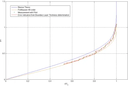
Figure 13.1: The velocity profile as measured with the Pitot tube with Rex= 3.26·105 (U=8m/s).
Figure 13.1 also shows the instability of the Silent Wind Tunnel at low velocities.
Figure 13.3: The velocity profile as measured with the Pitot tube with Rex= 4.88·105 (U=12m/s).
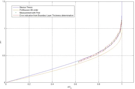
Figure 13.5: The velocity profile as measured with the Pitot tube with Rex= 1.02·106 (U=25m/s).
We observe an unpredicted trend in the velocity profile. The shape of the velocity profile appears to curve with increasing Reynolds number. The deviation can be caused by a combination of an error in the boundary-layer thickness determination and some error in the determination of the free stream velocity. A slight variation of 0.1m/s in the measured free stream velocity will result in a less curved velocity profile. It could also be caused by disturbances in the flow. Therefore the measurement with a free stream velocity of 25 m/s (Rex = 1.02·106) was repeated (at a different span of the plate) to
Figure 13.6: The second measurement on the velocity profile as measured with the Pitot tube with Rex = 1.02·106 (U=25m/s).
13.1.1 The Stagnation Pressure along the Span of the Plate
[image:64.595.76.523.192.413.2]The Pitot tube was placed along the span of the plate to measure the stagnation pressure. For every measurement point, the distance between the plate and Pitot tube was set identical. The measurement starts at 5 cm from the center of the plate and ends at 15cm from the center of the plate. The pressure was measured at 2.0 mm and 2.5 mm from the surface of the plate. The result of the measurement is shown in Figure 13.7.
Figure 13.7: The stagnation pressure along the span of the plate
The pressure measurement shows that the velocity is not constant along the span of the plate at the measured velocity for 25 m/s (Rex= 1.02·106) and therefore the flow is not uniform in this direction.
These changes are presumably due to anomalies of the surface of the plate, possibly also indicating the development of so-called turbulent wedges. The difference between the stagnation pressures is also plotted. The difference shows that when one would determine the velocity profiles at the measurement points, the resulting velocity profiles are not equal as Figure 13.5 and 13.6 already showed.
13.1.2 The Boundary-Layer Thickness
The boundary-layer thicknesses that are determined from the Pitot measurements are shown below.
Rex xδRe1x/2 (Blasius=4.92) 3.26·105 5.01
4.07·105 4.56 4.88·105 4.77 6.11·105 4.45 1.02·106 4.76 & 5.25
[image:64.595.219.374.597.669.2]13.1.3 Turbulent Flow Measurement
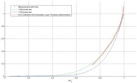
[image:65.595.66.537.196.481.2]The velocity profile in a turbulent boundary layer has also been measured. The result is shown in Figure 13.8. Turbulence was induced with a turbulator strip placed just downstream of the leading edge. With a very sensitive microphone it has been determined that there was indeed turbulent flow. However, the flow over the plate was not fully turbulent. A small area downstream of the leading edge still showed laminar flow behaviour. The result of the turbulent flow measurement is compared with the power law velocity profile. The 1/5th power law appears to fit the measurement results best.
13.2 The Velocity Boundary-Layer Measurement with the Hot Wire Anemometer
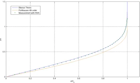
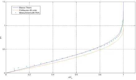
Figures 13.9 - 13.13 show the velocity profiles which have been measured with the HWA. The position of the HWA relative to the leading edge is the same as the position of the Pitot tube, a distance of x=0.62m from the leading edge. With the HWA it was very difficult to determine the distance from the plate since the HWA should not touch the plate. Therefore the HWA was placed increasingly closer to the plate until the measured voltage increased again, indicating that the wire was losing heat to the plate. From this starting position, the velocity was determined in steps of 0.1mm. Because of the difficulty in measuring the exact distance, the results have been fitted to the velocity profile according to Blasius. This does not change the shape of the graph but only shifts it in the y-direction.
[image:66.595.64.538.289.567.2]The measurements at U=8m/s and U=10m/s are plotted starting at a distance of 0.1mm from the plate. The measurements at U=12m/s, U=15m/s and U=25m/s are plotted starting at a distance of 0.2mm from the plate. The measurements for U=12m/s and U=15m/s do not show the behaviour close to the plate and thus the starting distance was set at a longer distance from the plate.
Figure 13.9: The velocity profile as measured with the Hot Wire with Rex= 3.26·105 (U=8m/s).
Figure 13.10: The velocity profile as measured with the Hot Wire with Rex= 4.07·105 (U=10m/s).
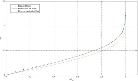
[image:67.595.62.535.416.698.2]Figure 13.12: The velocity profile as measured with the Hot Wire with Rex= 6.11·105 (U=15m/s).
Figure 13.13: The velocity profile as measured with the Hot Wire with Rex= 1.02·106 (U=25m/s).
The measurement for Rex= 1.02·106 (U=25m/s) starts at a distance of 0.2mm from the plate to fit
[image:68.595.78.518.401.659.2]13.2.1 The Boundary Layer Thickness
The determined boundary layer thicknesses from the Hot Wire measurement are shown in the table below. In general, the Hot Wire measurements are closer to the Blasius Theory than the Pitot tube measurements.
Rex δxRe 1/2
x , Pitot δxRe 1/2
x , Hot Wire 3.26·105 5.01 4.92 4.07·105 4.56 5.08 4.88·105 4.77 4.89 6.11·105 4.45 5.08 1.02·106 4.76 & 5.25 5.9
Table 2: The measured boundary layer thickness from both measurements (Blasius Theory = 4.92)
13.3 The Drag Force
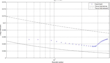
[image:69.595.74.521.425.681.2]The results of the drag force measurements are shown below. Information about the load cell, which was used to determine the drag force, can be found in Appendix C.4. The results show transition at a quite high Reynolds number, which is not as expected. According to the theory and XFOIL simulations, the critical Reynolds number at which transition should occur is at approximately 500,000 whereas in the present experiment transition occurs at a Reynolds number of about 3,000,0000. A possible cause is the streamwise pressure gradient for which the results are represented in section 13.4. The measured drag coefficient for laminar flow is observed to be slightly higher than the value from theory, which is most likely caused by the interaction of the side walls of the wind tunnel with the boundary layer on the plate.
Figure 13.14: The drag coefficient measured using the load cells