Periodic Wall Blow/Suction Perturbation Evolution in Turbulent Boundary Layer

(1)

Periodic Wall Blow/Suction Perturbation Evolution in

Turbulent Boundary Layer

*

Gangli Hao1,2, Nan Jiang1,3#

1_{Department of Mechanics, School of Mechanical Engineering, Tianjin University, Tianjin, China,} 2_{Shijiazhuang University of Economics, School of Engineering, Shijiazhuang, China,}

3_{Tianjin Key Laboratory of Modern Engineering Mechanics, Tianjin, China,}

Email: [email protected], #_{[email protected]}

Received July 12, 2012; revised August 12, 2012; accepted August 19, 2012

ABSTRACT

Time sequence signals of instantaneous longitudinal and normal velocity components at different longitudinal and nor-mal positions in a turbulent boundary layer have been finely measured simultaneously by IFA300 constant temperature anemometer and double-sensor hot-wire probe with sampling resolution higher than the frequency that corresponds to the smallest time scale of Kolmogorov dissipation scale before/after introducing artificial periodic blow/suction pertur-bation. The period-phase-average technique is applied to extract the periodic waveforms of artificial perturbation from instantaneous time sequence signals of longitudinal and normal turbulence background. Experimental investigation is carried out on the attenuation characteristics of periodic perturbation wave with different frequency along longitudinal direction and normal direction in a turbulent boundary layer. The amplitude distributions of longitudinal and normal disturbing velocity component for different perturbation frequencies are measured at different downstream and normal positions in turbulent boundary layer. The amplitude growth rate of artificial periodic perturbation wave is calculated according to flow instability theory. The experimental results are compared and in consistent with the theoretical and numerical results.

Keywords: Artificial Periodic Perturbation; Blow/Suction; Turbulent Boundary Layer; Hot-Wire Anemometry

1. Introduction

Since Kline (1967) [1] discovered the coherent large- scale low-speed streak structure for turbulence produc-tion in the near wall region of turbulent boundary layer, Whether the evolution of burst is related to near wall flow conditions or outer flow conditions is not given a clear conclusion. At the beginning, it was generally con-sidered streak structures and burst processes are the fea-ture phenomena in the near wall region influenced only by wall conditions directly, and it is independent of flow conditions in the outer region. Blackwelder (1972) [2] discovered that the movements in the viscous layer are strongly correlated with that in the outer region. Offen et al. [3] (1974)’s experiments also indicated that the burst

is deeply influenced by the outer flow. This is reasonable to explain the existence of large-scale vortex in the tur-bulent boundary layer and the energy source for turbu-lence generated by bursts. Rao [4] and Kim [5]

normal-ized the average burst cycle by using boundary layer’s external parameters (boundary layer thickness  and free flow velocity U_) and found that the normalized

average burst cycle is independent of the Reynolds num-ber. Laufer [6] concluded that TU  5 by

2 _0.65 0.7

T Tu_ Re_ 5 in the range of

and corroborated his experimental results. This discovery led the researches to emphasize on the relationship be-tween inner boundary layer and outer boundary layer. The experimental results of Rao [4], Kim [5] and Offten [3] showed that the generation of burst is related to the outer flow of boundary layer, which can explain rea-sonably the existence of large-scale vortex in the turbu-lent boundary layer and the energy source of turbulence production from burst, but the researches of Chamber [7], Willmarth [8], Luchick [9], and Shu [10] are more in-clined to the inner parameter’s impact on the coherent structure burst, they believed that the impact of wall shear is more direct and important. The debate on whether the burst temporal scale is impacted by outer or inner flow conditions is essentially on the generation and maintenance mechanism of burst. The occurrence and evolution of burst plays a key role in the generation and



_ _ _{500 R}_ _e _₁₀4



*_{This work was jointly supported by the National Natural Science}

Foun-dation of China (Grant Nos. 10832001 and 11272233), National key basic research and development program (plan 973) (NO. 2012CB-720101). This work was jointly supported by Hall of Hebei province science and technology of China (11213947).

(2)

maintenance of turbulence and the transportation of tur-bulence energy, thereby studies on the flow conditions influencing the generation and evolution of burst is of great significance.

Inspired by the success of imposing artificial periodic perturbation in lamina boundary layer transition experi-ment, adopting different methods to introduce artificial periodic perturbation to turbulent boundary layer and examining the influence of artificial periodic perturba-tions on the burst can solve, from another point of view, the problem of whether the burst time scale is influenced by outer or inner flow conditions. Hussain et al. [11,12]

introduced perturbation in the fully developed two-dimensional turbulent channel flow by using electromag-netic excitation method and got a result which is in agreement well with Landahl’s [13] linear theory. V. V. Kozlov, et al. [14] studied the developing process of

per-turbing wave in Poiseuille flow. Yao [15] introduced organized artificial perturbation in water channel ex-periments by mechanical vibrating ribbon, studied pre-liminarily the development and evolution of low-frequency perturbation wave along the longitudinal direc-tion and the influence of perturbadirec-tion in outer region on bursts in inner layer.

Theoretical researches are mainly focused on the de-velopment of sinusoidal wave perturbation by the method of lamina instability. Researches in this field started from M. Landahl’s waveguide model. The numerical results are in agreement with Willmarth’s [16] experimental results.

2. Experiment Technology and Apparatus

In this experiment, periodic artificial blow/suction per-turbations of different frequencies are introduced into a turbulent boundary layer through a spanwise slot by ex-citing a woofer vibrating under the wall in order to ma-nipulate the multi-scale flow structure in turbulent bound-

ary layer. The evolution and the influence of periodic blow/suction perturbation on the turbulent boundary layer are investigated experimentally. Periodic blowing and suction disturbance provides a simple method for wall-bounded turbulence control because the frequency and amplitude of blowing & suction disturbance is able to be quantified and adjusted easily and accurately.

Time sequence signals of longitudinal and normal ve-locity components at different longitudinal and normal positions in a turbulent boundary layer have been finely measured before/after introducing periodic blow/suction perturbation by IFA300 constant temperature anemome-ter and TSI-1243 double-sensor hot-wire probe with sampling resolution higher than the frequency that cor-responds to the smallest time scale of turbulence. In this paper, experimental results under the conditions of dif-ferent perturbation were compared and analyzed statisti-cally. Sampling frequency of the experiment is 20 KHz; measuring time for each sampling space point is 13.1072 seconds, and data volume is 262,144.

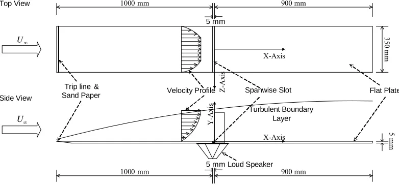
[image:2.595.102.493.539.723.2]

The experiment is carried out in the low-turbulent level wind tunnel of the Fluid Mechanics Laboratory of Tianjian University. The test section of wind tunnel is made of wood; the cross-section of the test section is a rectangular without corner, with 4500 mm in length, 450 mm in height, and 350 mm in width. Wind velocity in the test section can be continuously adjusted from 1.0 m/s to 40.0 m/s, and the background turbulent level is less than 0.07%. Experimental apparatus arrangement is shown in

Figure 1: the experimental flat-plate is 2000 mm in

length, 350 mm in width and 2 mm in thickness; the leading edge of the flat-plate, facing straightly the com-ing flow, is wedge-shaped; local perturbation is intro-duced through a spanwise slim slit of 5 mm longitudinal wide and 345 mm spanwise long on the smooth flat plate; the slim slit is located 1000 mm downstream away from

X-Axis

Z-A

xi

s

X-Axis

Y-A

xi

s

1000 mm

1000 mm 900 mm

900 mm

350

m

5 m

m



U

 U

Flat Plate Turbulent Boundary

Layer Spanwise Slot 5 mm

5 mm Top View

Side View

Loud Speaker Velocity Profile

Trip line & Sand Paper

(3)

the leading edge of the flat plate, The origin of the coor-dinate axes is located at the center point of the down-stream edge of the spanwise slot. The longitudinal direc-tion is x and the normal direction is y. A signal generator

is used to produce sinusoidal wave signals with control-lable frequency. The sinusoidal wave signals are ampli-fied by a power amplifier to power a 300 mm-diametered woofer periodically, introducing blow/suction perturba-tion airflow into the turbulent boundary layer, the ampli-tude of the perturbation is controlled by the amplifier’s power output.

TSI Company’s IFA300 constant temperature ane-mometer is used, together with CCTS-1193E automatic controlled three-dimensional coordinate frame and Ther- malpro software package to carry out the instantaneous velocity measurement automatically. The sensor is a TSI- 1243-T1.5 × type hot-wire probe with double slantwise hot-wires made of 5 μm diameter tungsten fine filament, and the probe is calibrated on the TSI-1128 hot-wire probe calibrator before used.

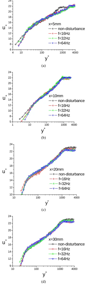
The mean velocity profiles with/without different fre-quency perturbations at two locations X = 5 mm X = 5

mm X = 10 mm X = 20 mm X = 30 mm downstream

re-spectively the disturbing source are plotted by inner variable unit in Figure 2 where uu u* and

*

yyu  are the normalized streamwise mean

veloc-ity and the distance from the wall by the skin friction velocity u* and the kinematics’ viscosity . The

un-disturbed longitudinal mean velocity profile fits to the Spalding law well. As for the disturbed profiles, lower mean velocities are found in the buffer layer where the logarithmic region is not affected. As the flow develops downstream, this phenomena gradually disappears and the disturbed velocity profiles recover to the undisturbed state at X = 30 mm. This implies that the effect domain of

blowing/suction periodic disturbance is limited and the blowing/suction periodic disturbance cannot be propa-gated downstream far away in turbulent boundary layer. The blowing/suction periodic disturbance is fused by the receptivity of turbulent boundary layer and decays gradually.

3. Experimental Results and Analysis

3.1. Experimental Data Analysis Methods

The eigenwaveform of the periodic artificial perturbation wave is educed by the phase-align period average tech-nique. It is convenient to represent the velocity field as a superposition of three parts:

j j j

u u u uj (1)

Here j = 1, 2, 3 stands for velocity components of three

directions, uj is the mean velocity over a long time

period, uj is phase average of periodic perturbation,

4 10 100 1000 4000

6 8 10 12 14 16 18 20 22 24

x=5mm

non-disturbance f=16Hz f=32Hz f=64Hz u+

y+

(a)

1 10 100 1000 4000

5 8 10 12 14 16 18 20 22 24

x=10mm

y+

(b)

10 100 1000 4000

10 12 14 16 18 20 22 24

u+ x=20mm_{non-disturbance}

f=16Hz f=32Hz f=64Hz

y+

(c)

10 100 1000 4000

9 12 14 16 18 20 22 24

x=30mm

y+

[image:3.595.332.512.89.682.2]

(d)

(4)

and uj corresponds to the background random

fluctua-tion. The mean velocity uj can be determined by

aver-age over a long time (long time averaver-age of uj and uj

are u_j = 0, uj = 0), uj can be obtained through the

phase-align period average method, and the phase aver-age of the instantaneous velocity then gives the sum of the mean and the organized wave. Denoting the phase average by , we have

j j

u u uj (2)

and then,

j j j j j

u  u u  u u (3)

The instantaneous velocity is measured at seven lon-gitudinal positions downstream from the perturbation source; the amplitude and eigenwaveform of the pertur-bation are measured by the phase-average technique.

It is usual to represent the two-dimensional perturba-tion wave as:



_{, ,}



1 _ˆ

 

  _ˆ

_{ }





2

i x c t i x ct

j

u x y t u y e u y e 

 

   



 _  _

 

  (4)

where * stands for complex conjugate, is the two- dimensional complex eigenmode, r i

 

ˆ

u y i

    is the complex wavenumber, r being the longitudinal wave

number and i the growth rate factor, and c cr ici

is the complex wave speed.

The perturbation velocity amplitudes at two different longitudinal stations x1, x2 with the same distance y

from the wall





 

_{ }





 

1 1

2

1

2

ˆ , ,

r i

i

i x t x ix1

x

u x y t u y e e u y e

u x y t u y e

   



  



 



 

 (5)

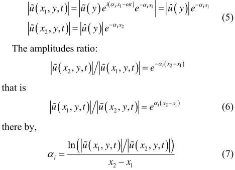
The amplitudes ratio:



 



2 1

2, , 1, , i

x x

u x y t u x y t e 

that is



 



2 1

1, , 2, , i

x x

u x y t u x y t e  (6)

there by,



 





1 2



2 1

ln , , , ,

i

u x y t u x y t

x x

 



 

(7)

If the perturbation amplitude increases along the lon-gitudinal direction, thus



 



2 1

2, , 1, , i 1

x x

u x y t u x y t e   (8)

that is



 



2 1

1, , 2, , i 1

x x

u x y t u x y t e   ,

and then  i 0 is obtained according to x2 x1 0.

If perturbation attenuations along the longitudinal di-rection, thus



 



2 1

2, , 1, , i 1

x x

u x y t u x y t e   (9)

that is



 



2 1

1, , 2, , i 1

x x

u x y t u x y t e   ,

and then  i 0 is obtained according to x2 x1 0.

It is known from above that for the same y value, wave

amplitudes at different longitudinal stations of x,

pertur-bation wave amplitude growth rate i can be calculated

from Equation (7).

3.2. Perturbation Wave Amplitude Distribution along x-y Plane

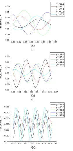
Figure 3 shows the period-averaged waveforms of

lon-gitudinal velocity component at five different vertical locations 10 mm downstream the blow/suction distur-bance source with different frequencies. It is can be seen that the period-averaged waveforms are typical sinusoi-dal disturbance.

Figure 4 are the perturbation wave amplitude

distribu-tions of 16 Hz, 32 Hz, 64 Hz across the turbulent bound-ary layer at different longitudinal stations downstream the disturbance source. The perturbation wave amplitude response in the outer region (y+ > 100) caused by the 16

Hz and 32 Hz perturbation is much larger than that in the near wall region (y+ < 100). It implies that the periodic

perturbation in the near wall region causes the response on the outer region, and it shows further the inner and outer boundary layer are not absolutely separated and they are sensible closely each other. The emergence of inner layer’s burst is intimately related to the outer boundary layer’s flow conditions.

While the 64 Hz perturbation distorts seriously in the turbulent boundary layer, the attenuations are relatively rapid, and fails to produce relatively large amplitude perturbation wave’s response in the outer region (y+ >

[image:4.595.55.289.462.632.2]

100), which is related to the inherent predominant ei-genmode of the turbulent boundary layer, as shown in

Figure 5. Figures 5(a)-(d) show, in different

longitudi-nal stations and the same normal position y+ = 12, before

(5)

0.00 0.01 0.02 0.03 0.04 0.05 0.06 0.07 -0.06

-0.04 -0.02 0.00 0.02 0.04 0.06

<u

(

16H

z

,t

)>

t(s)

y+=32.6 y+=36.0 y+=39.4 y+=42.8 y+=46.2

+ + + + +

(a)

0.00 0.01 0.02 0.03 0.04 0.05 0.06 0.07 -0.03

-0.02 -0.01 0.00 0.01 0.02 0.03

<u

(

32

H

z

,t

)>

t(s)

y+=33.8 y+=37.4 y+=40.9 y+=44.4 y+=47.9

+ + + + +

(b)

0.00 0.01 0.02 0.03 0.04 0.05 0.06 0.07 -0.015

-0.010 -0.005 0.000 0.005 0.010 0.015

<u

(

64H

z

,t

)>

t(s)

y+=34.6 y+=38.2 y+=41.8 y+=45.4 y+=49.0

+ + + + +

[image:5.595.62.314.79.598.2]

(c)

Figure 3. Phase average of periodic suction and blowing velocity components at different locations from the wall downstream the wave-maker 10 mm ((a) 16 Hz, (b) 32 Hz, (c) 64 Hz).

a = 7 (64 Hz). This shows that different frequencies periodic perturbations change the inherent frequency com-ponents of the velocity fluctuation in turbulent boundary layer. 64 Hz perturbation is the nearest frequency to the inherent main frequency of the velocity fluctuation in turbulent boundary layer, and the interaction with the

100 1000 10000

0.000 0.002 0.004 0.006 0.008 0.010 0.012 0.014 0.016

urm

s

y+

x=2.5mm x=5mm x=10mm

f=16Hz

(a)

100 1000 10000

0.000 0.002 0.004 0.006 0.008 0.010 0.012 0.014 0.016

urm

s

y+

x=15mm x=20mm x=30mm

f=16Hz

(b)

100 1000 10000

0.000 0.002 0.004 0.006 0.008 0.010 0.012 0.014

urm

s

y+

f=32Hz

(c)

100 1000 10000

0.000 0.002 0.004 0.006 0.008 0.010 0.012 0.014

urm

s

y+

x=15mm x=20mm x=30mm

f=32Hz

(6)

100 1000 10000 0.000

0.001 0.002 0.003 0.004 0.005 0.006 0.007

urm

s

y+

f=64Hz

(e)

100 1000 10000

0.000 0.001 0.002 0.003 0.004 0.005 0.006

0.007 x=15mm

x=20mm x=30mm

f=64Hz

u rm

s

y+

[image:6.595.71.277.83.409.2]

(f)

Figure 4. Decay of disturbance wave amplitude at different frequencies across turbulent boundary layer at different longitudinal stations downstream the disturbance source (a), (b) 16 Hz; (c), (d) 32 Hz; (e), (f) 64 Hz.

inherent frequency components in the turbulent boundary layer is the strongest. Thereby, the 64 Hz perturbation in turbulent boundary layer distorts seriously and attenua-tions rapidly, and cannot lead to large response in the outer region y+ > 100. Suppose, the frequency of the

per-turbation wave is 128 Hz (Scale 6), thus, it just fits the inherent frequency of the velocity fluctuation power spectrum in turbulent boundary layer, and its interaction with the frequency components in turbulent boundary layer is the strongest. It could attenuation most rapidly in turbulent boundary layer and cannot induce large re-sponse y+ > 100.

Yao [15] studied the evolution of periodic perturbation in the log law region of turbulent boundary layer in a water channel flow by the method of inducing artificial periodic perturbation through vibrating reed. The inher-ent frequency in the water channel flow is below 1 Hz, his perturbation frequency is 1 - 6 Hz, which is larger than the water channel flow’s inherent main frequency components. He found that the 1 Hz perturbation, which is approximate to the water channel flow’s inherent main frequency, distorts seriously, and attenuations rapidly.

0 2 4 6 8 10 12 14 16

-0.020.00 0.02 0.04 0.06 0.08 0.10 0.12 0.14 0.16 0.18 0.20 0.22 0.24 0.26 0.28 0.30 0.32 0.34

E

u

(a)

a

y+=12 x=2.5mm

non-disturbance f+=0.0094 f+=0.0188 f+=0.0376

(a)

0 2 4 6 8 10 12 14 16

-0.02 0.00 0.02 0.04 0.06 0.08 0.10 0.12 0.14 0.16 0.18 0.20 0.22 0.24

y+=12 x=5mm

non-disturbance f+_=0.0094

f+=0.0188 f+=0.0376

E

u

(a)

a

(b)

0 2 4 6 8 10 12 14 16

-0.02 0.00 0.02 0.04 0.06 0.08 0.10 0.12 0.14 0.16 0.18 0.20 0.22 0.24

y+

=12 x=10mm

non-disturbance f+=0.0094 f+

=0.0188 f+

=0.0376 E_u(a)

a

(c)

0 2 4 6 8 10 12 14 16

-0.02 0.00 0.02 0.04 0.06 0.08 0.10 0.12 0.14 0.16 0.18

y+=12 x=40mm

non-disturbance f+=0.0094 f+=0.0188 f+=0.0376

E

_u

(a)

[image:6.595.309.533.83.699.2]

a

(d)

(7)

Therefore, he concluded that the perturbation, which is most close to the inherent main frequency of the turbu-lent fluctuation energy in a turbuturbu-lent boundary layer and has the interaction with the frequency components in the turbulent boundary layer strongest, attenuations most rapidly, and the response in the outer region of turbulent boundary layer is the weakest. As the perturbations travel to the downstream, perturbation becomes weaken gradu-ally and its influence disappears when x = 40 mm, the

velocity fluctuation power spectrum recover to the case when no perturbation happens.

3.3. Perturbation Wave Amplitude’s Growth Rate Distribution in x-y Plane

Linear and nonlinear stability theoretical calculation in-dicates that there is no overall instability in turbulent boundary layer, for the turbulence is a dynamic equilib-rium and stable state. Perturbation waves at different frequencies under normal circumstances trend to attenua-tion. Figures 6-8 are respectively the amplitude growth

rate distribution of the perturbation wave of 16 Hz, 32 Hz and 64 Hz. The perturbation wave amplitudes trend to attenuation on the whole, that is, the overall amplitude growth rate of the perturbation wave is  i 0

0

i

, with sometimes local amplitude growth rate is   , and the development of the perturbation wave amplitude is not

1 2 3 4 5

20 40 60 80

-0.3200 -0.2400

-0.1600

-0.08000

0

0.08000 0.1600

0.2400

0.3200

X

[image:7.595.330.515.81.211.2]

Y

Figure 6. Amplitude attenuation rate in the (x, y) plane for 16 Hz perturbations.

1 2 3 4 5

20 40 60

80 -0.3200

-0.2400

-0.1600 -0.08000

0

0.08000

0.1600 0.2400

0.3200

X

[image:7.595.80.264.415.541.2]

Y

1 2 3 4 5

20 40 60 80

X

Y

-0.3200

-0.2400 -0.1600

-0.08000

0

0.08000 0.1600

0.2400

0.3200

always monotonous. The attenuation rate of 16 Hz and 32 Hz perturbation in the near wall region close to the perturbation source (y+ < 100) is weak, while in the outer

region is comparatively strong, but the attenuation rate along the longitudinal direction weakens gradually. The 64 Hz perturbation attenuations quickly in the whole flow field  i 0, because the 64 Hz perturbation is the most approaching to the inherent burst frequency of the turbulence and the interaction between the perturbation wave and turbulence is the strongest, perturbation wave attenuations most rapidly in turbulent boundary layer.

4. Conclusions

1) The inner and outer layers are not absolutely sepa-rated. They have the relationship of receptivity. The emergence of inner layer’s burst is intimatly related to the outer boundary layer’s flow conditions.

2) Perturbation waves at different frequencies under normal circumstances trend to attenuation. The amplitude of perturbation waves of different frequencies generally attenuations along the longitudinal direction and trends to become weaker gradually. But the perturbation wave amplitude does not always monotonously decrease with sometimes local amplitude growth rate is negative.

3) The 16 Hz and 32 Hz perturbation wave attenua-tions in a distance close to the perturbation source along the longitudinal direction, while their response is rela-tively strong in the area outside the logarithm law district. The perturbation at frequency that is the most approach-ing to the inherent burst frequency in turbulent boundary layer attenuations relatively rapid in the whole boundary layer.

4) The perturbation amplitude attenuation rate i

measured in this experiment is in agreement with the results analyzed and calculated by M. Landahl’s (1967) theory analysis.

REFERENCES

[image:7.595.80.265.579.706.2]

(8)

Runstadler, “The Structure of Turbulent Boundary Layer,”

Journal of Fluid Mechanics, Vol. 30, No. 4, 1967, pp.

741-774. doi:10.1017/S0022112067001740

[2] R. F. Blackweleder and R. E. Kaplan, “NATO-AGARD Conference Proceedings No. 93,” Technical Editing & Reproduction Ltd., London, 1972.

[3] G. R. Offen and S. J. Kline, “Combined Dye-Streak and Hydrogen-Bubble Visual Observations of a Turbulent Boundary Layer,” Journal of Fluid Mechanics, Vol. 62, No. 2, 1974, pp. 223-239.

doi:10.1017/S0022112074000656

[4] K. Rao Narasimha and M. A. Badri Narayanan, “The Bursting Phenonmena in a Turbulent Boundary Layer,”

Journal of Fluid Mechanics, Vol. 48, No. 2, 1971, pp.

339-396. doi:10.1017/S0022112071001605

[5] H. T. Kim, S. J. Kline and W. C. Reynolds, “The Produc-tion of Turbulence near a Smooth Wall in a Turbulent Boundary Layer,” Journal of Fluid Mechanics, Vol. 50,

No. 1, 1971, pp. 133-160.

doi:10.1017/S0022112071002490

[6] J. Laufer and M. A. Badri Narayanan, “Mean Period of the Turbulent Production Mechanism in a Boundary Layer,” Physics of Fluids, Vol. 14, No. 1, 1971, pp. 182- 197. doi:10.1063/1.1693271

[7] F. W. Chamber, H. D. Murphy and D. M. McEligot, “Lat-erally Covering Flow. Part 2, Temporal Wall Shear Stress,” Journal of Fluid Mechanics, 1982, pp. 127-403.

[8] W. W. Willmarth and L. K. Sharma, “Study of Turbulent Structure with Hot Wires Smaller than the Viscous

Length,” Journal of Fluid Mechanics, Vol. 142, 1984, pp.

121-149.

[9] T. S. Luchik and W. G. Tiedermann, “Time Scale and the Structure of Ejections and Bursts in Turbulent Channel Flow,” Journal of Fluid Mechanics, Vol. 174, 1987, pp.

529-577. doi:10.1017/S0022112087000235

[10] W. Shu and N. Tang, “Bursting Frequency in Turbulent Boundary Layers,” Acta Mechanica Sinica, Vol. 4, No. 4,

1988, pp. 291-296. doi:10.1007/BF02486661

[11] A. K. M. F. Hussain and W. C. Reynolds, “The Mechan-ics of an Organized Wave in Turbulent Shear Flow,”

Journal of Fluid Mechanics, 1970, pp. 41-241.

[12] A. K. M. F. Hussain and W. C. Reynolds, “The Mechan-ics of an Organized Wave in Turbulent Shear Flow. Part 2. Experimental Results,” Journal of Fluid Mechanics, 1972,

pp. 54-241.

[13] M. T. Landahl “A Wave-Guide Model for Turbulent Shear Flow,” Journal of Fluid Mechanics, 1967, pp. 29-

443.

[14] V. V. Kozlov and M. P. Ramazanav, “Development of Finite-Amplitude Perturbations in Posieuille Flow,” Fluid

Dynamics, Vol. 18, No. 1, 1983, pp. 30-33.

[15] “The Effect of Organized Wave Perturbations on Coher-ent Structure in Wall Turbulence,” Acta Mechanica

Sinica, Vol. 23, No. 4, 1991, pp. 47-54 (in Chinese).

[16] W. W. Willmarth and C. E. Wooldridge, “Measurements of the Fluctuating Pressure at the Wall beneath a Thick Turbulent Boundary Layer,” Journal of Fluid Mechanics,