http://dx.doi.org/10.4236/ijis.2014.43009
Adaptive Cascade Generalized Predictive
Control
Tao Geng
1, Jin Zhao
21Academy of Physics and Electroics, Henan University, Kaifeng, China
2Academy of Control Science and Engineering, Huazhong University of Science and Technology (HUST), Wuhan, China
Email: [email protected], [email protected]
Received 25 May 2014; revised 25 June 2014; accepted 2 July 2014
Copyright © 2014 by authors and Scientific Research Publishing Inc.
This work is licensed under the Creative Commons Attribution International License (CC BY). http://creativecommons.org/licenses/by/4.0/
Abstract
Cascade control is one of the most popular structures for process control as it is a special archi-tecture for dealing with disturbances. However, the drawbacks of cascade control are obvious that primary controller and secondary controller should be tuned together, which influences each other. In this paper, a new Adaptive Cascade Generalized Predictive Controller (ACGPC) is intro-duced. ACGPC is a method issued from GPC and the inner and outer controllers of a cascade system are replaced by one cascade generalized predictive controller, where both loops model are up-dated by Recursive Least Squares method. Compared with existing methods, the new method is simpler and yet more effective. It can be directly integrated into commercially available industrial auto-tuning systems. Some examples are given to illustrate the effectiveness and robustness of the proposed method.
Keywords
Adaptive Cascade Generalized Predictive Control, Model Identification, Cascade Control
1. Introduction
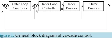
Figure 1. General block diagram of cascade control.
Previous researchers have proposed relay-based auto-tuning techniques to facilitate the design of cascade control systems. The methods proposed by Hang et al. [4] and Vivek and Chidambaram [5] need sequential ap- plication of the conventional relay-based auto-tuning approach, and are therefore still time consuming. The se-quential tuning procedure has been improved so that only single relay experiment is required for auto-tuning [6]- [9]. However, an off-line or ad hoc experiment must be performed in these methods. For example, Leva and Donida [6] performed test with relay cascaded to an integrator, and Mehta and Majhi [8] restricted the secondary controller to controller during the relay test. Besides the relay-based method, Visioli and Piazzi [10] proposed an automatic tuning method consisting of an open-loop test for cascade control system. Veronesi and Visioli [11] recently proposed simultaneous closed-loop automatic tuning method for cascade controllers. Their method evaluates the set-point step response of cascade control system.
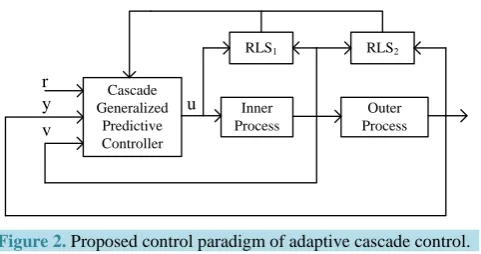
Whatever, based on the PID there are always two controllers needed to be configured. And obviously, the drawbacks of cascade control are obvious that primary controller and secondary controller should be tuned to-gether, which influences each other. If there is not a substantial difference in time constants, although this strat-egy can still be pursued, the loop design cannot be made independently and based on SISO techniques. So tun-ing is not intuitive: centralized configurations might be preferable. CGPC [12] [13] is a method issued from GPC and the inner and outer controllers of a cascade system are replaced by one cascade generalized predictive controller. In this control paradigm, there is only one controller configured. If the models of inner process and out process were known, the controller can be auto-configured. This paper proposed an adaptive CGPC cascade controller shown in Figure 2. The both loops model are SISO. And the model can be identified by the classical method, respectively.
2. GPC with Constraints
GPC adapts the model so-called Controlled auto regressive integrated moving average (CARIMA) model [14] [15].
( )
1( )
1 T z( )
1A z B z
−
− = − +
∆
y u e (1)
where, T z
( )
−1 is the model of noise, but it is commonplace to treat T z( )
−1 as a design parameter. Because it has direct effects on loop sensitivity and so better closed-loop performance will be got with a T z( )
−1 .Then, a general form of future predictions is
free
free P Q
= Γ∆ + = ∆ +
y u y
y u y (2)
And the followed can be derived
1
D B
C C−
Γ = (3)
where, D z
( )
−1 = ∆A z( )
−1T T
T T
P C P H
Q C Q H
= − Γ
= +
(4)
T
C is the toeplitz matrix of T z
( )
−1 and HT is the hankel matrix of T z( )
−1 [16]. Constraints on process inputs and outputs make the controller and consequently the entire closed-loop, nonlinear.Use the cost function and optimization
(
) (
)
2( )
(
)
2( )
2 2
1 1
y u
N N
y u
j j
J r k j y k j W j u k j W j
= =
=
∑
+ − + +∑
∆ + (5)Inner Loop Controller
Inner Process Outer Loop
Controller
Outer Process v
r
Figure 2. Proposed control paradigm of adaptive cascade control.
where, r k
(
+ j)
is j step ahead reference. Ny is receding horizon and Nu is control step. Wy, Wu is the output and input weight factor. Described in matrix form, the GPC with constraints is converted to be the opti-mization problem which is2 2 free T T min 2 s.t. 0 u y W W k
J r u y u
J S
C ∆
= − Γ∆ − + ∆
= ∆ ∆ + ∆ ∆ − ≤
u u u f u
u d
(6)
where, J is subject of the following constraints. Where S is positive definite and f , dk are time varying (dependent on the current state).
(
)
T T
free
, =
y u y
S= Γ W Γ +W f − Γ W r−y (7) The (6) is a standard quadratic programming with constraints. The constraints in GPC will be described as the following.
The Control Law without Constrains
Solve the J 0
u
∂ = ∂
The control law without constrains is derived as
(
)
1(
)
1 T T
free
y u y
S− W W − W
∆ = −u f = Γ Γ + Γ r−y (8)
Input move constraints
∆u is the lower bounds of input move constraints, and ∆u is the upper bounds of input move constraints.
1 1 k k k Nu + + − ∆ ∆ ∆ ∆ ∆ ∆ ≤ ≤ ∆ ∆ ∆ u u u u u u u u u
Which can be described in vector form as (9).
U U
∆ ≤ ∆ ≤ ∆u (9) And satisfy the matrix inequality (10)
0 I U I U ∆ ∆ − ≤ − −∆
u (10)
Input constraints
u is the lower bounds of input constraints, and u is the upper bounds of input constraints.
1 I k I I I ∆ − = ∆ +
u C u u
Inner Process Cascade Generalized Predictive Controller Outer Process r y v u
where, 0 0 0 I I I I
I I I
∆ = C . 1 1 k k k Nu + + − ≤ ≤ u u u u u u u u u 1 I k
U≤C ∆∆ +u Lu− ≤U (11) The corresponding linear inequalities are
1 1 0 I k I k U L U L ∆ − ∆ − − ∆ − ≤ − − + C u u C u
Output constrains
The output of plants always needs to be constrained in the bounds, as demand of process requirements. And they always are treated as soft constraints. Y is the lower bounds of output constraints, and Y is the upper bounds of output constraints.
free free free 0 Y Y Y Y Y Y ≤ ≤
≤ Γ∆ + ≤
Γ −
∆ − ≤
−Γ − +
y u y y u y (12)
If all constraints are satisfied, the (6) can be described as
I I I I ∆ ∆ − = −
Γ
−Γ C C C , 1 1 k k k U U U L U L Y P Q
Y P Q
− − ∆ −∆ − = − + − ∆ − − + ∆ + u d u u y u y (13)
qpOASES (quadratic program Online Active SEt Strategy) is an open-source implementation of the recently proposed online active set strategy, which was inspired by important observations from the field of parametric quadratic programming [16] [17]. The standard form is
T T
min 2
s.t.
J S lb ub lbA A ubA
∆ = ∆ ∆ + ∆ ≤ ∆ ≤ ≤ ∆ ≤
u u u u f
u u
The (6) can be converted to be in the qpOASES form. And the followed can be derived from (9), (11), (12)
ub
lb
U U
∆ ≤ ∆ ≤ ∆u
1 1
k I k
A
lbA ubA
U L U L
Y P Q Y P Q
− ∆ −
− −
≤ ∆ ≤
− ∆ − Γ − ∆ −
u C u
u
u y u y
Algorithm 1-GPC with constraints
1) Firstly, we can identify the plant A z
( )
−1 , B z( )
−1 , and Γ, , P Q can be calculated from (3), (4), Specify the factor Wy, Wu, T z( )
−1 , receding horizon Ny, control step Nu, bound of input U U, , bound of input rate ∆U, ∆U, bound of output Y Y, , calculate the lb ub A, , , initialize QProblem object (qpOASES).2) sample the output, update y.
3) update lbA ubA, and QProblem object, return the optimization value ∆u. 4) update ∆u, output ∆uk.
5) go to (2).
3. Cascaded Generalized Predictive Control
As shown in Figure 2, Inner process model is described as( )
1( )
1 1( )
11 1 1
T z
A z B z
−
− = − +
∆
v u e (14)
And outer process model is described as
( )
1( )
1 2( )
12 2 2
T z
A z B z
−
− = − +
∆
y v e (15)
Similar to Formula (1) and (2), future predictions for Formula (14) is
1 P1 Q1
∆ = Γ ∆ + ∆ + ∆v u u v (16)
means filter by T11 1 1 1 1 1
1 1 1
1 C CA B,P1 C HA B ,Q1 C HA A
− − −
Γ = = = −
1 1
1 1
1 1 1
1 1
T T
T T
P C P H
Q C Q H
= − Γ
= +
And the future predictions for Formula (15) is
2 P2 Q2
= Γ ∆ + ∆ +
y v v y (17)
means filter by T2
2 2 2 2 2 2
1 1 1
2 C CD B ,P2 C HD B,Q2 C HD D
− − −
Γ = = = −
2 2
2 2
2 2 2
2 2
T T
T T
P C P H
Q C Q H
= − Γ
= +
By substitution of Formula (16) into Formula (17)
(
)
2 1 P1 Q1 P2 Q2 2 1 2 1P 2Q1 P2 Q2 free
= Γ Γ ∆ + ∆ + ∆ + ∆ + = Γ Γ ∆ + Γ ∆ + Γ ∆ + ∆ + = Γ∆ +
y u u v v y u u v v y u y
where, Γ = Γ Γ2 1, yfree= Γ ∆ + Γ2 1P u 2Q1v+ ∆ +P2 v Q2y The control law without constrains corresponds with (8). The control law with constrains for intermediate output
3 3 3 3 free
free 3 3
P Q P Q
= Γ ∆ + ∆ + = Γ ∆ + = ∆ + ∆
v u u v u v
v u v
means filter by T11 1 1 1 1 1
1 1
1 1
1 1 1
1 1 1
3 3 3
3 3
, ,
D B D B D D
T T
T T
C C P C H Q C H P C P H
Q C Q H V v V
− − −
Γ = = = −
= − Γ
= + ≤ ≤
(19)
V is the lower bounds of intermediate output v constraints, and V is the upper bounds. By substitution of Formula (18) into Formula (19)
3 3 3
V ≤ Γ ∆ + ∆ +u P u Q v≤V The corresponding linear inequalities are:
3 3 3
3 3 3
0
V P Q V P Q
Γ
∆ − − ∆ − ≤
−Γ − + ∆ +
u v u u v 0 k ∆ − ≤
C u d
where, 3 3 I I I I ∆ ∆ − = −
Γ
−Γ C C C , 1 1 free free k k k U U U L U L V V − − ∆ −∆ − = − + − − + u d u v v
The control law with constrains is converted to be standard quadratic programming with constraints problem and can be solved by Algorithm 1.
4. Classical RLS Method
The SISO system can be identified by classical RLS method, which is described as followed.
[
]
[
]
T T 1 1 T 1 1 k k n mk - k -n k - k -m
y e
a a b b y y u u
= + = = θ φ θ φ (20)
means filter by T in Equation (1). where θ is a vector of adjustable model parameters and ek is the corresponding error at time k. The aim is to select θ so that overall modeling error is minimized. The clas-sical recursive least square algorithm is
-1
T T
1 1
T
k k-1 k k-1
1 +
ˆ =ˆ + ( ˆ )
k k k
k y µ µ − − = − − =
P φ φ P φ φ P
θ θ K θ φ
K Pφ
(21)
In the RLS algorithm, the Pk update equation Equation (21) is very sensitive to the truncation errors and there is no guarantee that Pk will always be positive and symmetric defined. The parameter identified by RLS will have biases from the true parameters, the stability and robustness of the algorithm is very poor. And then
k
P is revised as
(
T)
2 k = k + k
5. Verification on Proposed Scheme
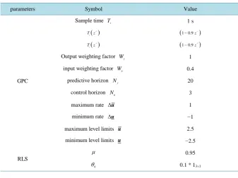
Two examples are presented here to illustrate the effectiveness of the proposed tuning method for cascade con-trol systems shown in Figure 2. The parameters of the ACGPC are in the Table 1.
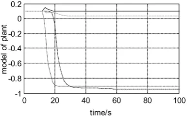
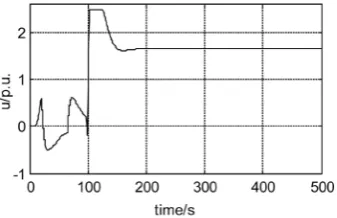
In simulation, there is an identification process at first 100 s. Both inner and an outer model are identified by the classical RLS, respectively. The final value of model identified by the RLS is shown in the Table 2 and Ta-ble 3, respectively. And the Figures 3-6 show model parameters estimated by RLS. There is rarely fluctuation in convergence of parameter estimated. Based on the model, the CGPC is applied to control the cascade system. The outer process outputs (primary outputs) of the control loops are presented in Figures 5-8. The figure clearly shows the CGPC have excellent transient performance. This implies that all the good properties of the cascade control are kept in the ACGPC. This behavior is specific to the cascade structures. And the ACGPC can auto- tune the CGPC.
Table 1. Numerical simulation parameters setting.
parameters Symbol Value
GPC
Sample time Ts 1 s
( )1 1
T z− ( 1)
1−0.9 z−
( )1 1
T z− ( 1)
1−0.9 z−
Output weighting factor Wy 1
input weighting factor Wu 0.4
predictive horizon Ny 20
control horizon Nu 3
maximum rate ∆u 1
minimum rate ∆u −1
maximum level limits u 2.5
minimum level limits u −2.5
RLS
µ 0.95
0
[image:7.595.124.471.227.736.2]θ 0.1 * 13×1
Table 2. Identification result of RLS for the real model.
Symbol Value
Inner loop model A1
[
1.0000 −0.9048]
Inner loop model B1
[
0.0952]
Outer loop model A2
[
1.0000 −0.9458]
[image:7.595.128.466.247.499.2]Outer loop model B2
[
0.03]
Table 3. Identification result of RLS for the real model.
Symbol Value
Inner loop model A1
[
1.0000 −0.8187]
Inner loop model B1
[
0.1813]
Outer loop model A2
[
1.0000 −0.9625]
Figure 3. Identification result of RLS for the real model
( )
1
[image:8.595.201.397.238.382.2]G s and G s2
( )
. [image:8.595.199.398.408.534.2]Figure 4. The control signals with and with control in-put constraints.
Figure 5. The tracking and regulation performance of the CGPC.
[image:8.595.199.399.568.694.2]Figure 7. The control signals with and with control in-put constraints.
Figure 8. The control signals with and with control in-put constraints.
• Example 1 The inner process is:
( )
11
10 1
G s s
= + The outer process is:
( )
20.6
20 1
G s
s
= + • Example 2
The inner process is:
( )
11
5 1
G s s
= + The outer process is:
( )
20.6
30 1
G s
s
= +
6. Conclusion
This paper developed an ACGPC method for the cascade control system, which gives the possibility to identify and control some different variables together. Both inner loop and outer loop process model, parameters can be identified using classical RLS method. Consequently, well-identified model based on CGPC can be applied to cascade control system. Finally, two examples were given to show the effectiveness of the proposed method. The method is very straightforward and has been integrated into an existing auto-tuning system. It is now being tested in an electrical drives system and the field results will be reported soon.
Acknowledgements
[image:9.595.215.384.84.193.2]ence Foundation of China with grant number 61273174.
References
[1] Pisano, A., Davila, A., Fridman, L., et al. (2008) Cascade Control of PM DC Drives via Second-Order Sliding-Mode Technique. IEEE Transactions on Industrial Electronics, 55, 3846-3854.
http://dx.doi.org/10.1109/TIE.2008.2002715
[2] Tsang, K.M. and Chan, W.L. (2008) Non-Linear Cascade Control of DC/DC Buck Converter. Electric Power Compo-nents and Systems, 36, 977-989. http://dx.doi.org/10.1080/15325000801960937
[3] Wolff Erik, A. and Skogestad, S. (1996) Temperature Cascade Control of Distillation Columns. Industrial & Engi-neering Chemistry Research, 35, 475-484.
[4] Hang, C.C., Loh, A.P. and Vasnani, V.U. (1994) Relay Feedback Auto-Tuning of Cascade Controllers. IEEE Transac-tions on Control Systems Technology, 2, 42-45. http://dx.doi.org/10.1109/87.273109
[5] Vivek, S. and Chidambaram, M. (2004) Cascade Controller Tuning by Relay Auto Tune Method. Journal of the Indian Institute of Science, 84, 89-97.
[6] Leva, A. and Donida, F.F. (2009) Autotuning in Cascaded Systems Based on a Single Relay Experiment. Journal of Process Control, 19, 896-905. http://dx.doi.org/10.1016/j.jprocont.2008.11.013
[7] Song, S., Cai, W. and Wang, Y.G. (2003) Auto-Tuning of Cascade Control Systems. ISA Transactions, 42, 62-72.
http://dx.doi.org/10.1016/S0019-0578(07)60114-1
[8] Tan, K.K., Lee, T.H. and Ferdous, R. (2000) Simultaneous Online Automatic Tuning of Cascade Control for Open Loop Stable Processes. ISA Transactions, 39, 233-242. http://dx.doi.org/10.1016/S0019-0578(00)00006-9
[9] Visioli, A. and Piazzi, A. (2006) An Automatic Tuning Method for Cascade Control Systems. Proceedings of the IEEE International Conference on Control Applications, Munich, July 2006, 2968-2973.
[10] Veronesi, M. and Visioli, A. (2011) Simultaneous Closed-Loop Automatic Tuning Method for Cascade Controllers.
Control Theory and Applications, 5, 263-270.
[11] Benyó, I. (2006) Cascade Generalized Predictive Control—Applications in Power Plant Control. University of Oulu, Oulu.
[12] Benyó, I. (2007) Cascade Generalized Predictive Controller: Two in One. International Journal of Control, 79, 866- 876.
[13] Clarke, D.W., Mohtadi, C. and Tuffs, P.S. (1987) Generalized Predictive Control—Part II. Extensions and Interpreta-tions. Automatica, 23, 149-160. http://dx.doi.org/10.1016/0005-1098(87)90088-4
[14] Clarke, D.W., Mohtadi, C. and Tuffs, P.S. (1987) Generalized Predictive Control—Part I. The Basic Algorithm. Auto-matica, 23, 137-148. http://dx.doi.org/10.1016/0005-1098(87)90087-2
[15] Rossiter, J.A. (2003) Model-Based Predictive Control-A Practical Approach. CRC Press, Washington DC, 54-58.
[16] Ferreau, H.J. (2009) qpOASES (Quadratic Program Online Active SEt Strategy) Version 2.0. http://www.qpoases.org/
currently publishing more than 200 open access, online, peer-reviewed journals covering a wide range of academic disciplines. SCIRP serves the worldwide academic communities and contributes to the progress and application of science with its publication.