A Dynamic Analysis of Educational Attainment, Occupational Choices, and Job Search

Munich Personal RePEc Archive

A Dynamic Analysis of Educational

Attainment, Occupational Choices, and

Job Search

Sullivan, Paul

Bureau of Labor Statistics

September 2006

A Dynamic Analysis of Educational Attainment,

Occupational Choices, and Job Search

Paul Sullivan

Bureau of Labor Statistics

September 2006

Abstract

This paper examines career choices using a dynamic structural model that nests a job search model within a human capital model of occupational and educational choices. Individuals in the model decide when to attend school and when to move between …rms and occupations over the course of their ca-reer. Workers search for suitable wage and non-pecuniary match values at …rms across occupations given their heterogeneous skill endowments and preferences for employment in each occupation. Over the course of their careers workers endogenously accumulate …rm and occupation speci…c human capital that af-fects wages di¤erently across occupations. The parameters of the model are estimated with simulated maximum likelihood using data from the 1979 co-hort of the National Longitudinal Survey of Youth. The structural parameter estimates reveal that both self-selection in occupational choices and mobility between …rms account for a much larger share of total earnings and utility than the combined e¤ects of …rm and occupation speci…c human capital. Eliminating the gains from matching between workers and occupations would reduce total wages by 30%, eliminating the gains from job search would reduce wages by 19%, and eliminating the e¤ects of …rm and occupation speci…c human capital on wages would reduce wages by only 2.7%.

Keywords: Occupational Choice, Job Search, Dynamic Discrete Choice, Human Capital

1 In

tr

ct

Over the course of their careers people choose how much education to obtain, which occupations to

work in, and when to move between …rms. Despite the interrelated nature of these choices, previous

research has generally examined educational and occupational choices separately from decisions

about job search. Empirical studies of occupational and educational choices are f tly based

on the framework of human capital models, which have taken the form of dynamic programming

models in recent work (Keane and Wolpin 1997, Lee 2005, Lee and Wolpin 2006). In these dynamic

human capital models workers endogenously accumulate education and occupation speci…c human

capital as they make optimal career choices, but all jobs are identical within an occupation. In

contrast to dynamic human capital models, an extensive job search literature has emphasized

the importance of job matching between workers and …rms in determining wages while generally

abstracting away from both occupational choices and human capital accumulation.1 MCall (1990)

and Neal (1999) depart from this trend by developing search models that incorporate occupations,

but these models do not include human capital accumulation.

The goal of this research is to further the understanding of how people make decisions about

educational attainment and employment by estimating a dynamic structural model of career choices

that incorporates the key features of a job search model within a dynamic human capital model

of occupational and educational choices. In the model, forward looking workers choose when to

attend school and when to move between occupations and …rms as they maximztheir discounted

expected utility. Search frictions such as randomness in job o¤ers and moving costs impede the

optimal allocation of workers across occupations and …rms. Over the course of their careers workers

endogenously accumulate general human capital in the form of education as well as occupation and

…rm speci…c human capital. The value of employment varies over the …ve occupations in the

economy because workers have heterogeneous skill endowments and preferences for employment

across occupations, and because the e¤ect of human capital on wages varies across occupations.

Workers search for suitable wage and non-pecuniary match values at …rms across occupations given

their innate skills and preferences and stock of human capital. Allowing for search based on

non-pecuniary utility general s the approach used in many search models which assume that workers

search only for wage match values.2

This paper contributes to a growing literature that demonstrates the value of using dynamic

discrete choice models to study employment and educational choices over the career. relevant

to the work presented here are the dynamic human capital models developed by Keane and Wolpin

(1997, 2001) and dynamic structural models such as Eckstein and Wolpin (1999) and B l l and

Hansen (2002) that focus on the endogenous accumulation of education. The model developed in

this paper expands on the occupational choice model of Keane and Wolpin (1997) by adding job

matching between workers and …rms, …rm speci…c human capital, heterogeneity in preferences for

employment in each occupation, and by expanding the number of civilian occupations from two to

…ve. Incorporating the human capital occupational choice approach to career dynamics along with

the …rm based job search approach within a uni…ed model is necessary to determine the relative

importance of each modelling approach in explaining career choices, wages, and total utility.

The parameters of the structural model are estimated by simulated maximum likelihood using

data from the 1979 cohort of the National Longitudinal Survey of Youth (NLSY). The likelihood

function follows directly from the recursive numerical solution to each individls dynamic

pro-gramming problem. The computational cost of estimation is substantial because simultaneously

modelling human capital accumulation, job search, and occupational choices creates a dynamic

programming problem that is challenging to solve. Estimation is made feasible by implementing an

interpolation method when solving the dynamic programming problem that modi…es the approach

2_{See Blau (1991), Hwang,}

ortensen, andReed (1998), and Dey and Flinn (2005) for examples of search models

that incorporate non-pecuniary job characteristics.

developed by Keane and Wolpin ( in a way that takes advantage of the special structure of

this model.

The career choice model nests a human capital model of occupational choices and a job search

model, so the structural parameter estimates provide direct evidence about the relative importance

of …rm and occupation speci…c human capital, job search, and heterogeneity in occupation

spe-ci…c skills and preferences in determining career choices, wages, and total utility. The parameter

estimates show that features of a dynamic human capital model and job search model are both

necessary to understand the evolution of wages and utility over the career. The potential percent

increase in wages caused by the acquisition of …rm speci…c human capital ranges from 9.5% to2

across occupations, and the potential wage gains from occupation speci…c human capital range from

essentiallyero to 17% across occupations.

3 _{The estimates of the e¤ects of human capital on wages}

indicate that search models that do not incorporate human capital accumulation are missing an

important source of wage growth. The potential wage gains from job search are alsoquite large. A

worker who is able to move from a 25th percentile …rm match to a 75th percentile match realies

a 45% increase in wages. Occupational choice models set in a human capital framework where all

jobs are identical within occupations are missing a key determinant of wage growth.

The structural model is used to conduct counterfactual simulations thatqantify the importance

of …rm and occupation speci…c capital, education, matching between workers and …rms, and

match-ing between workers and occupations in determinmatch-ing total earnmatch-ings and overall welfare. Previous

research has not been able to determine the relative importance of these factors because existing

models have not incorporated job search, occupational matching, and human capital accumulation

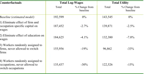
within a uni…ed model. The counterfactual simulations reveal that eliminating the returns to …rm

and occupation speci…c capital reduces total wage earnings by 2.7%. The wage gains resulting from

3_{Estimating the return to …rm tenure has been the subject of a large literature. See, for example, Altonji and} Shakotko (197), Topel (1991), and Dustmann andeghir (2005). Estimating the returns to occupation tenure has

received far less attention. See, for example, Kambourov andanovskii (2006) for instrumental variables estimates

utility maximiing mobility between …rms and occupations far exceed the wage gains from human

capital accumulation. The counterfactual simulations demonstrate that eliminating the wage gains

from job search reduces earnings in the simulated economy by 19%, while eliminating the gains

from matching between workers and occupations reduces total earnings by 30%. The total social

value of matching between workers and …rms, which includes pecuniary and non-pecuniary utility,

is 33% of total utility. The importance of both job search and occupational choices in determining

total earnings and utility highlights the value of jointly modelling these two key facets of the career

decision process.

The model is also used to determine the importance of permanent heterogeneity in skills and

preferences in determining lifetime utility relative to the importance of randomness in wage and

utility shocks, randomness in human capital improvement, and randomness in the arrival of

…rm-speci…c job matches. The results indicate that64%of the variation in lifetime utility is determined

by permanent heterogeneity. To provide some context for this result, Keane and Wolpin (1997) …nd

that90% of lifetime utility is determined by permanent heterogeneity in their career choice model

that does not consider the role of matching between workers and …rms in determining wages and

utility. Allowing for matching between workers and …rms, …rm speci…c human capital, and random

shocks to non-pecuniary utility reduces the relative importance of permanent heterogeneity in

determining lifetime utility, but its impact is still substantial.

The remainder of the paper is or !"d as follows. The next section discusses the data. Section

3 presents the model of career choices, and Section 4 discusses estimation. Section 5 presents the

structural parameter estimates, and Section 6 presents the results of the counterfactual experiments.

Section 7 concludes.

The parameters of the model are estimated using the 1979 cohort of the National Longitudinal

Survey of Youth (NLSY). This data set includes detailed information about the educational and

employment experiences of a nationally representative sample of 12,6$ 6men and women who were

%& ') % years old when …rst interviewed in 1979. Interviews were conducted annually up until %* *& +

and then biennially in the following years. The data provide a rich set of educational information

about each respondent, including dates of school attendance and dates of graduation and GED

receipt. Employment data include the duration of every employment spell over the sample period,

along with the corresponding wages, hours, and occupation for each employment spell. This

infor-mation allows for the identi…cation of transitions between employers and occupations, as well as

the patterns of wage changes over the career.

The NLSY consists of a nationally representative core sample, a military sample, and a

supple-mental sample that over-samples blacks, Hispanics, and economically disadvantaged whites. This

analysis uses only white men from the nationally representative core sample. Individuals who are

older than age sixteen in the …rst year of the NLSY are not used. Individuals remain in the data

set up to age thirty or until the observation is truncated at the …rst instance of missing information

about yearly labor force status or the occupation of a yearly job. , -spondents are dropped from

the sample if they provide insu¢ cient information to construct a history of educational attainment.

, -.pondents are also dropped from the sample if they ever serve in the military or work as a farmer.

The …nal sample consists of 1,023 men who remain in the sample for an average of 10.37 years,

resulting in 10,609“person y-e /.0of data.

The decision period in the model corresponds to a school year, which runs from September to

August.3

The data are aggregated using an approach similar to that of Keane and Wolpin (1997).

Yearly school attendance is assigned using detailed information on monthly school attendance and

grade completion. The methodology used to assign yearly school attendance consists of several

5

Yearly data is fre7uently used when estimating dynamic structural models. See, for example, Keane and Wolpin

steps. First, the amount of education accumulated by each sample member over the sample period

is determined using the variable that indicates the highest grade completed as of each interview

year. Then, starting in the …rst year, individuals are considered to be attending school if they

report attending school during the year and completing a grade by the next year. If this approach

fails to assign all the accumulated years of education, then the process is repeated using the weaker

:; <= > :ement that the person reports completing a grade or attending school during a year.?;ceipt

of a@ED is coded using yearly information on whether or not a person ever earned a@ED.

Yearly employment status is determined using the weekly labor force record. The yearly

em-ployment activity is the activity (a speci…c employer or unemem-ployment) in which the most weeks

were spent during the year. The number of weeks spent unemployed and employed full time at

each employer are counted for each decision year. Jobs consisting of less than twenty hours of work

per week are counted as time spent unemployed.5 The work activity in which the most weeks were

spent during the school year is coded as the yearly labor force activity. For example, suppose that

during a year a person works at …rm Afor 22 weeks, works at …rm B for 10 weeks, and spends 20

weeks unemployed. The primary activity for this year is working at …rm A, so working at …rm A

is coded as the yearly activity. The yearly occupation is the one corresponding to …rm A. @ >Aen

the assumption that employment is full-time, an individ=C EFs wage is converted into a yearly wage

by multiplying the hourly wage by 2,000 hours.

Transitions between …rms are identi…ed using the NLSY survey variables that indicate whether

or not a current employer is the same as an employer in the previous year. One unavoidable

cons; <=;nce of the aggregation of weekly data into yearly data is that yearly data understate the

number of transitions between …rms. The identi…cation of transitions between …rms is a key feature

of the model presented in this paper, so it is important to consider the e¤ects of aggregation on

the number of transitions between …rms present in the data. One way of assessing the e¤ects of

5_{Incorporating part time employment as a choice variable in the structural model is conceptually straightforward,} but it would increase the cost of estimation substantially.

aggregation is to compare the average number of jobs that a person holds over the sample period

using di¤erent levels of aggregation. Using the weekly NLSY employment record, the average

number of jobs is 11. When the data are aggregated to half-yearly, the average number of jobs falls

to 7. Using yearly data, the average number of jobs is 6. The e¤ects of aggregation are fairly large

when moving from weekly to half-yearly data, but relatively small when moving from half-yearly

to yearly data.6

The NLSY data provides information on occupational codes at the three digit level. The level

of detail provided in these codes raises HJestions about the proper de…nition of an occupation.

The human capital model presented in this paper suggests that an occupation should be de…ned

as a set of jobs that have common KL HJ N Kements in terms of skills and abilities. Based on this

de…nition, occupations should be de…ned in such a manner that within each group some portion

of an individual’s occupation speci…c abilities and accumulated skills will be transferable across all

jobs that fall into the group. Another important consideration is that the cost of estimating the

model increases substantially as the number of occupations increases, so using extremely detailed

occupational classi…cations is not computationally feasible. Based on these considerations,

occu-pations are aggregated into the …ve occupational groups listed in Table 1. Aggregating occuoccu-pations

into …ve groups is a lower level of aggregation than that found in existing research. OLPent dynamic

structural models of occupational choices such as Keane and Wolpin (1997) and Lee (2005) have

aggregated the data into only two occupations (blue and white collar). Lee and Wolpin (2006)

model both sectoral and occupational choices by allowing workers to choose between blue, white,

and pink collar employment in both the service and goods sectors, but they do not model job search

decisions.

6_{Hall (19}

Q2) provides a basis for comparison, reporting that workers, on average, hold 10 jobs over the course of

STU VWscrXptXvW YtatXstXcs

This section highlights the key characteristics of the data and provides descriptive statistics about

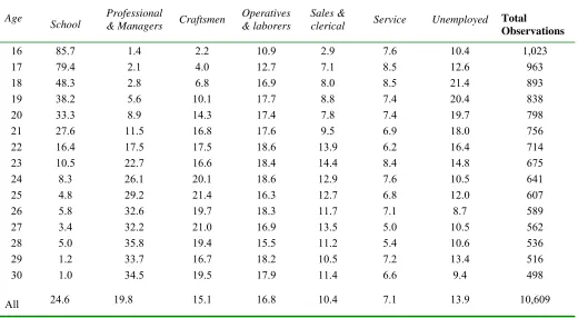
the career choices observed in the data. Table 2 shows the choice distribution by age. There are

1,023 people in the sample at age 16. This number declines fairly smoothly over time because some

observations are truncated at each age due to missing data. Approximately Z [ \ of the sample

attends school at age 16. School attendance takes a discrete drop to ]Z\at age^Z _the age where

most people have graduated from high school. As an alternative to high school graduation, 6.6%

of the sample reports earning a `ED at some point over the sample period. School attendance

declines steadily throughout the college ages and then drops to approximately 16% at age 22, the

normal college graduation age. School attendance declines to ]aZ\ by age 25, and continues to

decline at more advanced ages. Keane and Wolpin (2001) report abc gh jtatively similar relationship

between age and schooling using less highly aggregated data that divides each school year into

three segments. As school attendance declines with age, the percentage of people employed as

professional and managerial workers steadily increases from 1.]\ at age 16 to k]a5% at age 30.

In contrast, the percentage of people employed as service workers is relatively stable over time,

ranging between 5 and Z\a

The percentage of people unemployed is 10% at age 16. Unemployment rises to approximately

20% at ages ^Zt w^ before stabiljx jyg at close to 10% at ages w] and above. The large number of

people classi…ed as unemployed is due to the de…nition of school attendance used to classify people

as attending school. { |} gh h that a person must attend school and complete a grade to be coded as

attending school, so people who attend school and fail to complete a grade are classi…ed as

unem-ployed. Additionally, a person who is unemployed for 27 weeks during a year and employed for 25

weeks is classi…ed as unemployed, because his primary activity during the year was unemployment.

Keane and Wolpin (1997) report a similarly high rate of unemployment using slightly di¤erent

Table 1

Description of Aggregated Occupations

Aggregated Occupations

1970 Census Occupation Codes

Example Occupations

Professional, Technical,

Managers 001 - 245

Architects, Economists, Office Managers

Craftsmen 401 - 580 Carpenters, Electricians, Automobile Mechanics

Operatives & Non-farm Laborers 601 - 785 Butchers, Truck Drivers, Groundskeepers Sales & Clerical 260 - 395 Insurance Agents, Bank Tellers

Service 901 - 984 Janitors, Dishwashers, Nursing Aides

Table 2

Choice Distribution by Age

Age

School

Professional

& Managers Craftsmen

Operatives & laborers

Sales &

clerical Service Unemployed Total

Observations

16 85.7 1.4 2.2 10.9 2.9 7.6 10.4 1,023

17 79.4 2.1 4.0 12.7 7.1 8.5 12.6 963

18 48.3 2.8 6.8 16.9 8.0 8.5 21.4 893

19 38.2 5.6 10.1 17.7 8.8 7.4 20.4 838

20 33.3 8.9 14.3 17.4 7.8 7.4 19.7 798

21 27.6 11.5 16.8 17.6 9.5 6.9 18.0 756

22 16.4 17.5 17.5 18.6 13.9 6.2 16.4 714

23 10.5 22.7 16.6 18.4 14.4 8.4 14.8 675

24 8.3 26.1 20.1 18.6 12.9 7.6 10.5 641

25 4.8 29.2 21.4 16.3 12.7 6.8 12.0 607

26 5.8 32.6 19.7 18.3 11.7 7.1 8.7 589

27 3.4 32.2 21.0 16.9 13.5 5.0 10.5 562

28 5.0 35.8 19.4 15.5 11.2 5.4 10.6 536

29 1.2 33.7 16.7 18.2 10.5 7.2 13.4 516

30 1.0 34.5 19.5 17.9 11.4 6.6 9.4 498

All 24.6 19.8 15.1 16.8 10.4 7.1 13.9 10,609

Table 3 shows that there are di¤erences in the levels of inter-…rm and intra-…rm occupational

mobility. The relevant entries in each cell for this discussion are the top entries, which are

com-puted using the NLSY data.7 ~ €ility between occupations is more likely to occur when a person

switches …rms than when the person does not switch …rms. The age patterns in these two types

of occupational mobility are also  ‚ite di¤erent. Inter-…rm occupational mobility declines by 29%

from the youngest age group to the oldest, while intra-…rm occupational mobility declines byƒ „%.

The di¤erence in the age patterns between these two types of mobility suggests that opportunities

for intra-…rm occupational switches may become less …† ‡ ‚ ‡ˆt with age.

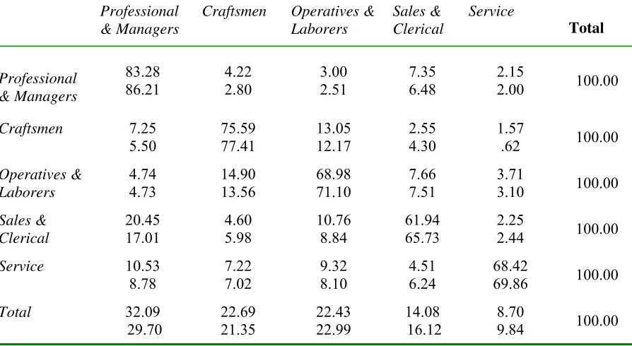
Table ƒ allows for a more detailed examination of mobility between occupations. Cell (i,j)

of this table (where i represents the row and j represents the column) gives the percentage of

employment spells in occupationi that are followed by a spell in occupationj. The relevant entries

for this discussion are the top entries, which are computed using the NLSY data. For example,

cell (2,1) indicates that a person employed as a craftsman has a 7.25% chance of becoming a

professional or managerial worker in the next year, conditional on being employed in the next year.

The diagonal elements of the occupational transition matrix in Tableƒare fairly large, indicating a

substantial amount of persistence in occupational choices. However, even at this relatively high level

of aggregation there is a substantial amount of occupational mobility. The diagonal elements show

that people employed as professional and managerial workers are least likely to switch occupations,

while sales and clerical workers are most likely to switch occupations.

Overall, the transition matrix is fairly symmetric, with the exception of the ‰ows of workers

between the sales and clerical and service occupations to professional and managerial employment.

Workers are much more likely to switch from sales and clerical or service employment to professional

and managerial jobs than in the opposite direction. The largest‰ow of workers between occupations

occurs from sales and clerical to professional and managerial employment.

7_{The bottom entries in the cells in Tables 3 and}

Šare computed using simulated data generated from the estimated

structural model. These entries will be discussed in detail later in the paper.

Table 3

Summary of Occupational Mobility by Age: NLSY Data (top entry) and Simulated Data (bottom entry)

Ages Conditional on Switching

Firms, % Switching Occupations

Conditional on not Switching Firms, % Switching

Occupations 16-21 57.64% 54.36% 29.94% 27.42% 22-25 50.09% 47.21% 26.85% 23.51& 26-30 40.76% 37.84% 17.61% 14.98% All Ages 49.78%

46.51%

24.69% 21.82%

Note: Probabilities are computed using all consecutive years of employment observed in the data for each age group. The top entry in each cell is computed using the NLSY data, and the bottom entry is computed using simulated data generated using the estimated structural model.

Table 4

Occupational Transition Matrix: NLSY Data (top entry) and Simulated Data (bottom entry)

Professional & Managers

Craftsmen Operatives &

Laborers Sales & Clerical Service Total Professional & Managers 83.28 86.21 4.22 2.80 3.00 2.51 7.35 6.48 2.15

2.00 100.00

Craftsmen 7.25

5.50 75.59 77.41 13.05 12.17 2.55 4.30 1.57

.62 100.00

Operatives & Laborers 4.74 4.73 14.90 13.56 68.98 71.10 7.66 7.51 3.71

3.10 100.00

Sales & Clerical 20.45 17.01 4.60 5.98 10.76 8.84 61.94 65.73 2.25

2.44 100.00

Service 10.53

8.78 7.22 7.02 9.32 8.10 4.51 6.24 68.42

69.86 100.00

Total 32.09

29.70 22.69 21.35 22.43 22.99 14.08 16.12 8.70

9.84 100.00

‹ Œ

c

c

ar

r

c

s

Each individuaš›s career is modeled as a …nite horiœon, discrete time dynamic programming problem.

In each year, individuals maximiœe the discounted sum of expected utility by choosing between

working in one of the …ve occupations in the economy, attending school, earning aED, or being

unemployed. Workers search for suitable wage and non-wage match values across …rms while

employed and non-employed given their skills and preferences for employment in each occupation.

Dual activities such as simultaneously working and attending school are also feasible choices.ž

The exact set of choices available in year t depends in part on the labor force state occupied in

the previous year. Each period, an individual always receives one job o¤er from a …rm in each

occupation and has the option of attending school, earning a  Ÿ  ¡ or becoming unemployed.

In addition, people who are employed have the option of staying at their current job during the

next year and may also have the option of switching occupations within their current …rm. While

employed, a worker receives eitherœ£ ¤ ¥or one opportunity to switch occupations at his current …rm. 9

Individuals observe all the components of the pecuniary and non-pecuniary rewards associated with

each feasible choice in each decision period and then select the choice that provides the highest

discounted expected utility.

Human capital enters the model through the endogenous accumulation of both …rm and

occu-pation speci…c work experience and education, which a¤ect wages and non-pecuniary utility¦ows.

Thus, workers choose to accumulate schooling, which is costly, in order to obtain higher utility in

the future. Jobs are also partly investment goods in the model because forward looking workers

realiœe that work experience a¤ects the distributions of wage o¤ers and non-pecuniary bene…ts that

they face.

§

Light (2001) …nds that omitting work experience gained while attending school produces an upward bias of 25%-¨ ¨% in the estimate of the return to schooling.

9

©any models of labor mobility ignore the possibility that workers may switch occupations within a …rm. Analysis

of the NLSY data presented in Section 2 suggests that that a signi…cant fraction of workers switch occupations without switching …rms.

ª«¬ ­t®¯®t° ±²³ct®´³

The utility function is a choice speci…c function of endogenous state variables(St), skill endowments

and preferences, and random utility shocks that vary over time, people, occupations, and …rm

matches. The variables inSt measure educational attainment, …rm and occupation speci…c human

capital, and theµ ¶· ¸¹ty of the match between a worker and …rm. To index choices for the non-work

alternatives, let s = school, g = GED and u = unemployed.10 _{Describing working alternatives}

º» µ ¶¹ ºes two indexes. Let eq=¼employed in occupationq½, whereq= 1; :::;5indexes occupations.

Also, letnf =¼working at a new …r¾½, and of =¼working at an old …º ¾¿ ½Combinations of these

indexes de…ne all the feasible choices available to an individual. The description of the utility

Àows is simpli…ed by de…ning another index that indicates whether or not a person is employed,

so letemp=¼employ»Á½. De…ne the binary variabledt(k) = 1 if choice combination kis chosen at

timet, wherekis a vector that contains a feasible combination of the choice indexes. For example,

dt(s) = 1indicates that schooling is chosen at timet, anddt(s; e3; nf) = 1indicates attending school

(s) while employed in the third occupation (e3) at a new …rm (nf). Dual activities composed of

combinations of any two activities are allowed subject to the logical restrictions outlined in Section

3.1.2.

ÂÃ ÄÃ Ä Choice Speci…c Utility Flows

This section outlines the utility Àows corresponding to each possible choice. The utilityÀow from

choice combination k is the sum of the logarithm of the wage, wit(k), and non-pecuniary utility,

Hit(k), that person ireceives from choice combination kat timet,

Uit(k) =wit(k) +Hit(k): (1)

1 0_{There is no uncertainty in the receipt of a}

ÅED in the model. If an individual decides to earn aÅED, he receives

one. In reality, people must pass a test to earn aÅED. Tyler et al (2000) report that roughly 70% of people pass the

The remainder of this section describes the structure of the wage and non-pecuniary utility Çows

in more detail.

3.1.1a Wages. The log-wage of worker iemployed at …rm j in occupationq at time tis

wit=wq(Sit) + q_i + ij +eijt: (2)

The term wq(Sit) represents the portion of the log wage that is a deterministic function of the

work experience and education variables in the state vector. The occupation speci…c subscript q

allows the parameters of the wage ÈÉ ÊË ÌÍÎ Ï to vary over occupations. For example, the e¤ect of

education on wages may di¤er by occupation. The term q_i represents the random component of

workeriÐs wages that is common across all …rms in occupation q. This term allows people to have

comparative advantages in their occupation speci…c skill endowments.11 _{The permanent}

worker-…rm productivity match is represented by _ij. This term Ñ ÈÇects match speci…c factors that are

unobserved by the econometrician and a¤ect the wage of worker i at …rmj. True randomness in

wages is captured byeijt. All of the components of the wage (wit) are observed by the worker when

a job o¤er is received.12

3.1.1bNon-pecuniary Utility Flows. Non-pecuniary utilityÇows are composed of a determin-istic function of the state vector, …rm speci…c match values, person speci…c preference heterogeneity,

and random utility shocks. De…ne 1ÒÓ Ôas the indicator function which isÈÉÊË Õ to one if its

argu-ment is true andÈÉÊËÕtoÖ Èro otherwise. The non-pecuniary utility Çow

ÈÉÊËÌÍÎ Ïis

Hit(k) = [h(k; Sit)] +

h

s i1Òs

×k Ô+

u i1Òu

×k Ô+

P5

q=1

q i1Òeq

×k Ô

i

(3)

+"ikt:

1 1_{Keane and Wolpin (1997) show that heterogeneity in skill endowments is an important determinant of the choice} between blue and white collar employment.

1 2_{See Berkovec and Stern (1991) for another model where the}

Øuality of the match is revealed when drawn. In

contrast, Jovanovic (1979) develops a model where agents learn about matchØuality over time.

The …rst term in brackets represents theÙÚ Ûuence of the state vector on non-pecuniary utilityÛows

and is discussed in more detail in the following paragraph. The second term in brackets captures

the e¤ect of person speci…c heterogeneity in preferences for attending school ( s_i), being unemployed

( ui), and being employed in occupation q ( q

i). The non-pecuniary occupation match value, q i,

represents the random component of person iÜs preference for working in occupationq. This term

captures variation in the value that people place on job attributes such as the physical or mental

demands of a job or the risk of injury that is common across jobs in each occupation. Stinebrickner

(2001) shows that preference heterogeneity is an important determinant of occupational choices

at the narrow level of choosing between a teaching or non-teaching job. However, this type of

heterogeneity in preferences has not been extended to broader models of occupational choice. The

term s_i allows for heterogeneity in the cost of schooling caused by unobserved traits such as ability

or motivation that may alter the utility cost of attending school. The …nal term,"ikt, is a shock to

the non-pecuniary utility that personireceives from choice combination k at timet.

The remaining portion of the non-pecuniary utility function contains the non-pecuniary

em-ployment and non-emem-ployment utility Ûows along with the schooling cost function. This utility

ÛowÝÞ ßà áÙâÚ is speci…ed as

h(k; Sit) = hP

5

q=1 q(Sit)1ãeqäkå+ ij1ãempäkå i

æ çè

+Cs(Sit)1ãsäk; emp =äkå+C

sw_(S

it)1ãsäk; empäkå

+b(Sit)1ãuäkå+C

g_(S

it)1ãgäkå:

The term in brackets contains the occupation and …rm speci…c non-pecuniary utility Ûows. The

occupation speci…c portion of thisÛow, q(Sit), is a function of the state vector that is allowed to

vary over occupations. This speci…cation allows the e¤ect of state variables such as education on

employment utility to vary by occupation. The …rm speci…c non-pecuniary match value for person

of employment at each …rm that a¤ect the employment utility êow and are not observed by the

econometrician. For example, job attributes such as commuting distance, relationships with

co-workers, and availability of fringe bene…ts may all a¤ect the value of a job, and their value may

di¤er across people. Non-wage matching of this type has not been incorporated in previous models

of occupational choice.13 _{The second line of}

ë ìíationîcontains the schooling cost function. There

are two schooling cost functions, one for attending school while not employed, Cs_(S

it), and one

for attending school while working at the same time,Csw(Sit).1ï

The two schooling cost functions

allow for the possibility that attending school is more costly while employed. The …nal components

of the non-pecuniary utilityêow are the deterministic portions of the value of leisure enjoyed while

unemployed,b(Sit), and the cost function for earning a ðED, C

g_(S it).

3.1.2 Constraints on the Choice Set

The structural modeling approach ñëìíòñëó a detailed speci…cation of the labor market constraints

that determine an individíô õös choice set in each year. First, consider the case of an individual who

enters time period t having not been employed in the previous year. At the start of the year the

individual receives …ve job o¤ers, one from a …rm in each of the …ve occupations in the economy.

÷ëøall that a job o¤er consists of the wage and non-pecuniary value that the worker places on the

job. The individual also observes all components of the rewards associated with attending school,

earning a ðED, being unemployed, and all feasible combinations of these choices. 15

1 3_{Non-wage job characteristics have been shown to be an important determinant of mobility. Bartel (19}

ù2) reports

that non-wage job characteristics are an important determinant of job úuitting behavior. Blau (1991) rejects a

reservation wage search model in favor of a reservation utility model where hours of work a¤ect utility. 1û

The model does not consider the e¤ect of borrowing constraints on educational attainment, since this addition would render an already complicated model completely intractable. Keane and Wolpin (2001) present evidence that although borrowing constrains are severe, relaxing these constraints has little impact on educational attainment. Cameron and Taber (2003) examine this issue using a number of di¤erent empirical approaches and consistently …nd that given the current policy regime, there is no evidence of ineüciencies in the schooling market created by

borrowing constraints.

1 5_{In this model workers always have the option of returning to their current job, although the o¤ered wage will} change because each job receives a new random shock in each year (e_ijt). Thus, transitions into unemployment

are utility maximiýing responses to shocks. This framework is adopted in many papers such as Berkovec and Stern

(1991), Keane and Wolpin (1997), and Lee and Wolpin (2005). An alternative framework allows for a job destruction (layo¤) probability and allows workers to always stay at the existing job at the previous wage. Eckstein and van den Berg (2006) discuss these two alternative models and conclude thatþThere is no aspect of the data that would force

Any dual activity is a feasible choice, subject to the following restrictions. Earning a G

must be part of a joint activity, so the single activitydt(g) = 1is not a feasible choice. In addition,

earning aGED is dropped from the choice set after high school graduation orG receipt. Finally,

unemployment and employment are mutually exclusive choices. Given these restrictions, the choice

set for individuals who are not employed when they enter period tis

D_tne = f[dt(s); dt(u); dt(u; g)];[dt(ei; nf); i= 1; :::;5]; (5)

[dt(q; ei; nf); q=s; g; i= 1; :::;5]g:

The …rst three terms correspond to the feasible non-employment opportunities, the next …ve terms

correspond to employment in each of the …ve occupations, and the …nal ten terms are the feasible

combinations of employment and education.

Next, consider the feasible choices for a person employed in occupation q:At the start of period

t the individual receives one new job o¤er from a …rm in each of the …ve occupations and has the

option to attend school, earn aG or become unemployed.

16 _{In addition, an employed individual}

always has the option of remaining at his current …rm and staying in his current occupation (q).

Job o¤ers from new occupations at the current …rm are received randomly, where workers receive

eitherz or one such o¤er per year. Let j denote the probability that a worker receives an o¤er

to work in occupationj at his current …rm, where j6=q. Let nq be the probability that a worker

employed in occupation q does not receive an o¤er to switch occupations within his current …rm.

This structure implies that in each period a worker always has the option of switching occupations

if he switches …rms, but mobility between occupations within a …rm is restricted by the receipt of

employment, unemployment, and the observed dynamic transitions among these states and the observed accepted wages."

1 6_{One possible althernative speci…cation of the model would be to incorporate job o¤er probabilities from each} occupation so that in any given time period, an individual may not receive job o¤ers from all …ve occupations. One could then attempt to estimate these o¤er arrival rates. However, because only accepted wages and transitions are observed in the data, this alternative model is completely observationally equivalent to the one presented in this

paper. For example, suppose that in the data we observe that laborers rarely ever become professionals. When we only observe transitions and accepted wages it is impossible to distinguish a world where laborers infrequently receive

job o¤ers. This feature of the model is intended to capture the fact that the scope for mobility

between occupations within a …rm is likely to be more limited than opportunities for mobility into

new occupations when a person also switches …rms.

Within-…rm occupation switch o¤er probabilities are identi…ed by functional form assumptions

and the transition rates between occupations observed in the data. The model imposes the

re-striction that the distribution of the random components of job o¤ers is the same for internal and

external job o¤ers. iven this restriction, within-…rm occupation switch job o¤er probabilities are

identi…ed by the fact that in the data, within-…rm occupational switches are observed less tly

than transitions between occupations when a person moves to a new …rm.17

The choice set for a worker employed in occupation q who receives an o¤er to switch to

occu-pation j at his current …rm is

De_t(j) =D

ne

t ;[dt(eq; of); dt(s; eq; of); dt(g; eq; of)];[dt(ej; of); dt(s; ej; of); dt(g; ej; of)]: (6)

If an o¤er to switch occupations within the current …rm is not received, then the …nal three choices

are not available to the agent. Let De

t(0) denote this twenty-one element choice set.

3.1.3 State Variables

The endogenous state variables in the vector St measure human capital and the uality of the

match between the worker and his current employer. Educational attainment is summari d by

the number of years of high school and college completed, hst and colt, and a dummy variable

indicating whether or not a has been earned,gedt:Possible values of completed years of high

school range from0to4, and the possible values of completed college range from0to5, where …ve

years of completed college represents graduate school. Work experience is captured by the amount

of …rm speci…c human capital (f ct) and occupation speci…c human capital (oct) in the occupation

that the person worked in most recently. Let O_t 2 [1;2; :::;5] indicate the occupation in which a

1 7_{See Canals and Stern (2002) for a discussion of a similar identi…cation issue that arises in a simple search model.}

person was most recently employed. LetLt be a variable that indicates a pe s previous choice,

whereLt=1; :::;5 refers to working in occupations one through …ve, Lt= 6 indicates attending

school full time, andLt= 7 indicates unemployment.

iven this notation, the state vector is St = hst; colt; gedt; f ct; oct;Ot; Lt; t; t: Including

both …rm and occupation speci…c human capital as state variables causes problems because the

s eof the state space s kly becomes intractably large due to the fact that the model incorporates

job search, occupational choices, and educational choices. In order to keep the model tractable,

only human capital in the most recent occupation is included in the state space even though this

eses a strong assumption about the transferability of human capital across occupations and the

depreciation of human capital.18

However, age e¤ects are included in the wageeations to proxy

for general human capital that has value in more than one occupation.

In addition to assuming that only human capital in the most recent occupation a¤ects wages,

a second approach is taken to further reduce the sie of the state space. Assume that …rm and

occupation speci…c human capital each take on P values, so that the possible values of human

capital arranged in ascending order are

f ct F C =f c(1);:::; f c(P)

oct OC =oc(1);:::; oc(P):

After each year of work experience, with probability human capital increases to the next level,

and with probability (1 ) human capital does not increase.19 There are separate skill increase

probabilities for …rm and occupation speci…c capital, and the rates of skill increase are also allowed

1

Ideally, one would allow for cross-occupation experience e¤ects in the wage e uation, which would re uire adding measures of previous occupation speci…c human capital to the state space. Unfortunately, allowing for these e¤ects would render an already extremely computationally demanding estimation problem completely infeasable given cur-rent computer technology. Due to the si!e of the state space, along with the large number of parameters in the model,

estimating the model presented in this paper is only possible using interpolation methods and parallel processing techni ues. In addition, it is necessary to have access to a large parallel computing cluster to estimate the model in any reasonable amount of time. #iven these considerable di¢ culties, I leave the inclusion of cross-occupation

experience e¤ects as an extension for future research. 1 9_{Brown and Flinn (200}

to vary across occupations. The skill increase parameters are $

k

f; ko; k = 1; :::;5%, where the

subscripts f and o refer to …rm and occupation speci…c capital, and k indexes occupations. The

human capital transition probabilities ( ’s) are known by agents in the model. Upon entering a

new occupation, octis reset to the …rst level. Similarly,f ct starts at the …rst level in the …rst year

of employment at a …rm. The &'() of the state space is signi…cantly reduced when P is a small

number relative to the possible values of years of work experience, but the model still captures the

human capital improvement process. In this work, P = 3. Sections 5.1 and 5.2 present evidence

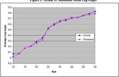
that the discrete approach to modelling human capital provides parameter estimates that …t the

observed patterns in wage growth in the NLSY extremely well.20

This method of modelling human capital has the advantage of making it possible to include both

…rm and occupation speci…c human capital in the state space at a fraction of the cost of keeping

track of actual years of experience at a …rm or in an occupation, because work experience could

range from ()ro to …fteen years in this model. In models of this type with large state spaces, an

alternative approach would be to place relatively low upper bounds on state variables, or omit some

of them entirely. The approach presented here is appealing from a practical standpoint because it

makes estimation feasible, but it is also consistent with the theory of human capital. The number

of years of completed work experience is generally included as an explanatory variable in wage

regressions only as a proxy for the unobservable level of human capital that actually a¤ects wages.

Viewing increases in human capital as a stochastic event is consistent with this idea, because it

2 0_{In a note about this paper Pavan (2006) comments that this model only allows for}

“restrictive wage growth

patterns.*However, in fact this approach to modeling human capital is+uite‡exible relative to approaches commonly

used in the literature, such as a+uadratic speci…cation. This approach allows wage growth pro…les to be concave

or convex, and heterogeneous across occupations. In addition, the model allows for ex post heterogeneity in the returns to human capital because“unlucky*individuals may never transition to a higher level of human capital over

their career, but“lucky*individuals may experience rapid wage growth. Random human capital improvements also

impact mobility because unlucky individuals will be more likely to switch jobs that lucky individuals. Pavan (2006) also allows for ex post heterogeneity by assuming that …rm and occupation speci…c human capital improvements follow a random walk with drift. However, one key di¤erence between the two approaches is that in Pavan,s model

at the start of a worker,s career there is no ex ante heterogeneity in expected wage growth because expected wage

allows for the possibility that years of work experience may vary for people with a given level of

human capital.

3.2 The Optimization Problem

Individuals maximi.e the present discounted value of expected lifetime utility from age 16 (t= 1)

to a known terminal age, t = T . At the start of his career, the individual knows the human

capital wage function in each occupation, as well as the deterministic components of the utility

function. An individual also knows his endowment of market skills ( /s) and occupation speci…c

non-pecuniary match values ( /s). Future reali.ations of …rm speci…c match values ( /s and /s)

and time and choice speci…c utility shocks ("/s ande/s) are unknown. Although future values are

unknown, individuals know the distributions of these random components. Individuals also know

the current values of all variables in the state vector, St, as well as the probability that human

capital will increase in the next period, conditional on employment ( k_f; ko; k= 1; :::;5).

The maximi.ation problem can be represented in terms of alternative speci…c value functions

which give the lifetime discounted expected value of each choice for a given set of state variables,St.

Variation in the structure of the value functions comes from di¤erences in the utility 0ows across

states, and di¤erences in the choice set across states. 3 57 9:ding the choice set, there are only

two relevant categories of states: employed (including joint employment activities), and all other

choice combinations. While people are employed, the possibility of mobility between occupations

within their current …rm implies that the value function will be structured di¤erently than when

non-employed, because the employed value function must incorporate the value of internal job

o¤ers. The value function and utility0ow5; <9= >?@ Aare functions of the state vector, St, but this

argument is suppressed for brevity of notation.

The value function for an individual with discount factor employed in occupation q is the

period,

Vt(eq; l) =Ut(eq; l) +

X

k6=q

kEZtek+ [ nqEZteq]; q = 1; :::;5; l=of; nf: (7)

TheEZek

t terms represent the expected value of the best choice in periodt+1, conditional on receipt

of an o¤er to work in occupation k at the workBC Ds current …rm. The expectations are taken over

the random components of the choice speci…c utilityEows, which are the random utility shocks and

match values, F"; e; ; H. The expectation is also taken over …rm and occupation speci…c human

capital,(f cand oc)since human capital evolves stochastically.21

Consider the …rst summation inBIJ KL Mon 7. Each term in the sum corresponds to the probability

that a job o¤er to work in a new occupation at the current …rm is received (sokN=q), multiplied

by the corresponding expected value of the best option next period. For each occupationq it must

be the case that P_j6=q j + nq = 1: The structure of the value function is similar to the model

presented by Wolpin (1992) in that both models allow the arrival of some types of job o¤ers to be

random, which implies that the values of future choices must be weighted by job o¤er probabilities.

Wolpin (1992) estimates job o¤er probabilities for unemployed and employed job searchers, in

contrast to the intra-…rm job o¤er probabilities estimated in the present model.

The individual elements of the EZek

t terms are the time t+ 1value functions for each feasible

choice,

EZ_tek = EmaxFVt+1(s); Vt+1(u); Vt+1(u; g);[Vt+1(ei; nf); Vt+1(m; ei; nf);

m=s; g; i= 1; :::;5;]; Vt+1(eq; of); Vt+1(s; eq; of); Vt+1(g; eq; of);

Vt+1(ek; of); Vt+1(s; ek; of); Vt+1(g; ek; of)H: O PQ

In the remainder of the paper, I will refer to these expected values asSEmaxT. The …nal term in

the employed value function corresponds to the case where an individual does not receive an o¤er to

2 1_See

Uust and Phelan (1997) for an example of another dynamic programming model where agents face uncertainty

about how the state vector will evolve over time.

switch occupations within his current …rm. In this case, switching occupations without switching

…rms is not possible, so the expected value of the best choice at timet+ 1is

EZ_teq = EmaxVVt+1(s); Vt+1(u); Vt+1(u; g); (9)

[Vt+1(ei; nf); Vt+1(m; ei; nf); m=s; g; i= 1; :::;5];

Vt+1(eq; of); Vt+1(s; eq; of); Vt+1(g; eq; of)W:

The value function for an individual who is not currently employed is simpler because mobility

within a …rm is obviously not possible for people who are not employed. The value function is

Vt(p) =Ut(p) + EZtsu; p=VsW;VuW;Vu; gW (10)

The corresponding expected value of the maximum term is

EZ_tsu = EmaxVVt+1(s); Vt+1(u); Vt+1(u; g); (11)

Vt+1(ei; nf); Vt+1(m; ei; nf); m=s; g; i= 1; :::;5W;

which consists of all feasible combinations of schooling, unemployment, and new job o¤ers.

Agents making career decisions use the value functions to determine the optimal educational

and employment choices in each period. Each period, a person observes all of the components of

the utilityXows of each feasible choice, and then calculates the value of each choice usingYZ [\ ]^_ `a

7 through 11. He then chooses the option with the highest discounted expected value.22

2 2_{A related model is developed by Pavan (2006), who presents a model of search across …rms and careers. Pavan} must make a number of assumptions to make his model tractable because he de…nes careers using very detailed three-digit occupation and industry codes. Some of the key di¤erences between the two papers are: 1) His model imposes the restriction that expected wage growth pro…les are identical across all occupations. In contrast, the results in this paper suggest that expected wage growth due to human capital accumulation varies widely across occupations, and that this heterogeneity has important implications for wage growth. 2) Education is exogenous in Pavanbs model, and

also is restricted to have the same e¤ect on wages across all occupations. These assumptions simplify the model, but as a result his model is unable to account for the fact that educational and occupational choices are made jointly. 3) There is no on the job search in Pavanbs model, while there is on the job search in the model presented in this paper.

In his model workers must choose to leave their jobs before observing a new o¤er, while in contrast this paper allows workers to observe their current job o¤er and the outside job o¤ers before making a mobility decision. In Pavanbs

model workers will leave bad matches, but the model is unable to account for wage growth resulting from workers receiving an extremely good secuence of job matches, because once workers have found a good match they will be

unwilling to leave that match to take a chance on receiving a better o¤er. As a result, his model predicts that 2d3

3.3 Solving the Career Decision Problem

Estimating the structural parameters of the modelr j kl mres solving theon p mtmuv p mon problem faced

by agents in the model. The …nite hormu owdynamic programming problem is solved by backwards

recursion. Assume that there is some age,T , after which no choices are made, and another age,T

at which the agent dies. Then, evaluating the value functions from T to T is straightforward,

because the value function for each choice is simply a sum of one period expected utility yows.

{mven the value functions at age T ;the value functions can be solved backwards recursively for all

t < T using j klations 7 through 11. Before considering the solution of the model in more detail,

it is useful to specify the distributions of the random components of utilityyows.

3.3.1 Distributional Assumptions

Assume that …rm speci…c match values and randomness in wages are distributed i.i.d normal:

ij v N(0; 2), ij v N(0; 2), and eijt v N(0; 2e). The …rm speci…c pecuniary and

non-pecuniary match values are part of the state space because the value function associated with a

job depends on the wage match value ( _ij) and non-wage match value ( _ij) for workeriat …rm j.

The distributions of these variables are continuous, which causes a problem because the state space

becomes in…nitely large when continuous variables are included. This problem is solved by using a

discrete approximation to the distributions of wage match values ( ij) and non-wage match values

( _ij) when solving the value functions and computing the likelihood function.

Assume that the random choice-speci…c utility shocks are distributed extreme value, with

dis-in every occupation, because he does not model comparative advantages across occupations. As a result, all sortdis-ing across occupations and mobility between occupations in his model is caused by random wage shocks. Therefore, it is unlikely that his model is able to match the distribution of workers across occupations, mobility patterns between occupations, or the wage distribution in each occupation. 5) Pavan|s model does not allow for non-pecuniary utility

to impact career choices. 6) His model does not incorporate unemployment. Still, Pavan|s model is richer than mine

in two dimensions. First, he considers the more general topic of career choice, rather than the occupational choices considered in this paper. He also uses the very detailed three-digit occupation and industry codes to de…ne careers, as opposed to …ve broad occupational groups. It is likely that using …ve broadly de…ned occupational categories understates mobility. However, it should be noted that one problem with using three-digit codes is that they are known to be extremely noisy. For example, a validation study by }ellow and Sider (19~3) …nds that only 5~% of

three-digit occupation codes are correctly recorded, so using three-digit codes will lead to a large number of false transitions between occupations.

tribution functionF(") = exp €exp(

"₎

, and with variance

2 2

=6:The assumption that the"‚s

are distributed extreme value simpli…es the computation of the value functions and choice

proba-bilities.

It remains to specify the distributions of the occupation speci…c skill endowments ( ‚s) and

preferences ( ‚s). Using an approach similar to Heckman and Singer (19ƒ„ …† Keane and Wolpin

(1997), and Stinebrickner (2001), the joint distribution of skill endowments and preferences is

speci…ed as a discrete multinomial distribution. Let i =

1

i; :::;

5

i;

1

i; :::;

5

i; si; uibe the vector

of skill endowments and preferences that are known to the agent at age sixteen.

Assume that there are M types of people, each with a di¤erent endowment of skills and

pref-erences,  m; m = 1; :::; M. De…ne m as the proportion of the mth type in the population.

Endowment heterogeneity is unobserved to the econometrician, but assume that we do know that

there are M types of people. This ˆexible assumption about the joint distribution of skills and

preferences allows for a wide range of patterns of comparative advantages in skills and heterogeneity

in preferences. As the number of types of people,M, becomes large, this approach can approximate

any joint distribution of skills and preferences arbitrarily well.

3.3.2 Calculating the Value Functions

This section discusses the details of the solution to the dynamic programming problem. The

major complication arises from the fact that as the model is speci…ed the Emax integrals do not

have closed form solutions. In many dynamic programming models, researchers assume that the

only randomness in utilityˆows is choice speci…c, independent over time, and distributed extreme

value.23 A cons‰Š ‹ ‰Œce of this assumption is that the Emax integrals have a simple closed form.

However, the unappealing cons‰Š ‹ ‰nce of this assumption in this application is that it rules out

job matching in wages and non-wage utility ˆows. Job matching in wages has been shown to be

empirically important in dynamic models such as Žer  ‘”ƒ„… and Berkovec and Stern (1991),

2 3_{See, for example,}

and is the basis of job search models.

To the extent that mobility decisions are based on non-wage factors, the addition of matching

in non-wage utility—ows to the career decision problem will contribute to the understanding of the

causes of transitions between …rms and occupations. This work allows for job matching e¤ects in

both wage and non-pecuniary utility by using simulation methods to evaluate the high dimensional

integrals ˜ ™š ›œ ˜ed to calculate Emax. Berkovec and Stern (1991) avoid having to use simulation

methods because they assume that people know their future job match values with certainty.

Allow-ing for uncertainty in future˜ ™žœ Ÿ  œons of job match values provides a more complete description

of the factorsœ ¡ —uencing mobility between …rms.

At this point it is useful to partition the vector of error terms, excluding ", into two sets. Let

t = £ ; ; e¤ be the set of errors whose future realiŸations are unknown to the agent at time t;

and de…ne the joint density of these errors asf( t). ¥™call that the vector of skill endowments and

preferences is i =£

1

i; :::;

5

i;

1

i; :::;

5

i; si; ui¤. Consider calculating the expected value of the best

choice available next period for a person who is employed in the current time period. Conditional

on t and …rm and occupation speci…c human capital (f ct and oct), the expected value of the

maximum has a closed form solution because of the assumption that"is distributed extreme value,

E max

dt2Dt

£V(dt) +"¦ t; i; oct; f ct¤ = ( + ln[ P

dt2Dt

exp(V(dt¦ t; i; oct; f ct)

)]) (12)

= (dt¦ t; i; oct; f ct);

whereV(dt) =V(dt) ", is Euž ™ ˜§s constant, and is a parameter of the extreme value

distribu-tion. Letf(¨)represent the density of the variable in parentheses. Integrating over the distributions

of t,f ctandoctprovides the unconditional expected value of the best choice available next period

for each endowment type,

E max

dt2Dt

£V(dt)+"¦ i¤=

Z Z Z

©©© Z

(dt¦ t; i; oct; f ct)f( t)d t f(f ct)df ctf(oct)doct: (13)

joint density f( t). In this work, R = 40.2¬

The integral over the distribution of human capital

is simply a probability weighted sum because the distribution of human capital is discrete. Let r

index simulation draws, and the simulated integral is simply the average of­® ¯ °± ²³´13 over theR

draws,

E max

dt2Dt

µV(dt) +"¶ i· = 1

R R

X

r=1

P

X

h=1

Pr[f ct=f ct(h)¶f ct 1]

P

X

z=1

Pr[oct=oct(z)¶oct 1]

(dt¶

r

t; i; oczt; f cht): ¸¹ º»

The other Emax terms found in the value function calculations are also approximated using this

method.

The major computational burden of solving the model arises from the fact that the Emax

func-tions must be simulated at each point in the state space over the agen±¼s entire time hori½on. When

the number of points in the state space is large, as it is in this model, evaluating the value function

becomes very time consuming. Several methods to reduce the computational expense of evaluating

value functions in dynamic programming models have been developed in recent years. For

exam-ple, ¾¯¿t (1997) proposes a method that uses ranÀ³Á²½°± ²³n to break the curse of dimensionality,

Keane and Wolpin (19º» use a linear regression to interpolate value functions, and Brien, Lillard,

and Stern (2006) interpolate value functions using a weighted average ofÃÄ Å³s­Ãpoints in the state

space.

This paper employs an interpolation algorithm that follows along the lines of the one developed

by Keane and Wolpin ¸¹Â º». As in Keane and Wolpin ¸¹Âº»Ævalue functions are simulated at a

fraction of the state space and interpolated using a regression at the remaining points in the state

space. This paper implements a new regression function that takes advantage of the assumption

that the error term " is distributed extreme value. If the only source of randomness in the model

was the error term", then the expected value of the maximum would have the closed form solution

2Ç

Antithetic acceleration is used throughout estimation to reduce variance of the simulated integrals. SeeÈeweke

(19É É) for a discussion of antithetic acceleration, and Stern (1997) for a review of the applications of simulation

shown in ÊË ÌÍ ÎÏon 12. This is not the case in this model due to the existence of the wage match

values ( ), non-wage match values ( ), and random wage shocks (e), but it suggests the following

functional form for the interpolating regression,

E max

dt2Dt

ÐV(dt) +"Ñ = !0t+!1t ( + ln[ P

dt2Dt

exp(V(dt))]) (15)

= !0t+!1t (dt):

The parameters!0t and!1t are estimated by OLS, and allowed to vary over time. This regression

function has the desirable theoretical property that it converges to the exact solution for Emax as

; ; and e approach 0. In addition, it also satis…es the theoretical restrictions on the Emax

function outlined in ÒcFadden (1Ó ÔÕ Ö× Another important property of this regression function is

that the regressor is de…ned at every point in the state space even if the set of feasible state points

varies over the state space, as it does in this model. In contrast, the regression function proposed

by Keane and Wolpin (199Ø Öuses the value functions corresponding to each element in the choice

set separately as regressors, which creates a missing data problem when the choice set is state

dependant.25

During estimation, the value functions are simulated at approximately1%of the state space and

interpolated at the remaining points. The regression function …ts the data very well. Throughout

estimation, theR2_{from the interpolating regression remained between:95and:99:Experimentation}

shows that the actual and interpolated value functions di¤er by approximately 1%on average.

4

Estimation of The Structural Model

The parameters of the model are estimated by simulated maximum likelihood ÙÚÒL) using the

career history data from the NLSY. This section begins by specifying functional forms for the

utilityÛowÊËÌÍÎÏÜ ÝÞ× It concludes with a derivation of the likelihood function and a discussion of

2 5_{One solution to this problem would be to use a di¤erent interpolating regression for each feasible choice set in} the state space. Depending on the exact details of the model, this approach has two potential drawbacks: 1) small sample sißes in each individual regression, 2) the need to estimate a large number of interpolating regressions.

the methods used to maxiàáâã the likelihood function.

4.1 Further Model Speci…cation

Before discussing the details of estimating the parameters of the structural model, it remains to

specify the wageãä åæ çáons, non-pecuniary utilityèowãä åæ çáéê ë, and job o¤er probabilities in more

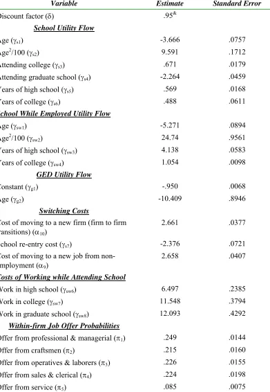
detail.

4.1.1 Wage and Utility Flow Equations

This section de…nes the deterministic portion of the utility function. The deterministic portion of

the occupation speci…c human capital wage function is

wq(Sit) = q1ageit+

q

2age 2

it=100 + q

3hsit+

q

4colit+

q

51[ageit ì17]+ (16)

q

61[ageití18îageitì21] +

q

7gedit

+ q81[f cit=f c(1)] + q91[f cit =f c(2)] + q101[f cit =f c(3)]

+ q111[ocit =oc(1)] + q121[ocit=oc(2)] + q131[ocit=oc(3)]:

The parameters q8 and

q

11 are …xed at âã ïé since they are not separately identi…ed from the

constant in the wage eäuation. 26

Let N Ft be a dummy variable indicating whether or not the individual is in his …rst year of

employment at a …rm after being employed at a di¤erent …rm in the previous period. Let hdt

and cdt represent dummy variables that indicate receipt of a high school or college diploma. The

non-pecuniary utilityèowãäåæçáéêfor occupationq is

q(Sit) = q1ageit+

q

2age 2

it=100 + q

3(hsit+colit) +

q

4ocit+

q

5f cit+

q

6hdit (17)

+ q7cdit+

q

8gedit+

q

91[Lit>5] +

q

10N Fit q = 1; :::;5:

The inclusion of explanatory variables in the employment non-pecuniary employmentèow eä

ua-tions allows observable variables to have a direct impact on employment utility in addition to any

2 6_{The inclusion of direct age e¤ects in the wage e}

ðuations follows the approach of Keane and Wolpin (1997). They