Improvisation to the R* Tree kNN Join Principles in Distributed Environment

Improvisation to the R*-Tree kNN Join Principles in

Distributed Environment

P.Xavier

Sacred Heart College Tirupattur

India

F.Sagayaraj Francis

Pondicherry Engineering College Puducherry

India

ABSTRACT

This paper identifies the scope for improvement in the execution of baseline kNN join algorithms in a distributed environment. Improvements are suggested and the improved methods are applied in performing kNN joins on R*-Trees. The effectiveness of the proposed improvements have been experimentally verified and presented.

General Terms

Database Systems, Multidimensional Querying, Distributed Systems.

Keywords

R*-Trees, kNN join, Hadoop, Mapreduce, z- values.

1.

INTRODUCTION

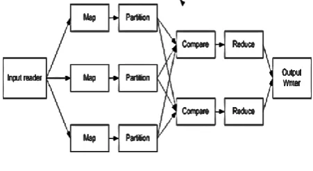
We are in an age where the data that are generated is voluminous, varied, complex and come at a rate and from places that are challenging to data management and data processing systems. It was obvious that the traditional Database Management Systems and the data processing and analyzing systems found it difficult to cope with such tremendous demands. The advent of Hadoop and Mapreduce [1] provided the opportunity for the management and processing to go distributed. Hadoop is a distributed computing framework, where clusters with many computing and storage facilities are dynamically formed. The management of the clusters are transparent to the users. Mapreduce is a programming paradigm for Hadoop distributed computing framework.

Figure 1 Mapreduce overview

A Mapreduce program consists of a pair of user defined map

and reduce functions. The map function is invoked for every record in the input data sets and produces a partitioned and sorted set of intermediate results. The reduce function fetches sorted data, from the appropriate partition, produced by the map function and produces the final output data. Conceptually, they are: map(k1, v1) → list(k2, v2) and

reduce(k2, list(v2)) → list(k3, v3). To reduce the network

traffic caused by repetitions of the intermediate keys k2

produced by each mapper, an optional combine function for

merging output in map stage, combine(k2, list(v2)) → list(k2,

v2), can be specified. An overview of Mapreduce is given in

Figure 1.

Figure 2 A sample R-Tree and the corresponding spatial objects in 2D

R-Tree [2] is data partitioned multi-dimensional indexing technique. Figure 2 gives a sample Tree. The original R-Tree has undergone a lot of changes since its inception. R*-Tree [3] is one such efficient version of R-R*-Tree. The R-R*-Tree leaves hold the multidimensional objects in n-dimensional rectangular spaces called Minimum Bounding Rectangles (MBRs). The higher level nodes progressively group the MBRs in the lower level into bigger MBRs and form a hierarchy of MBRs resulting in an R-Tree. In this paper the terms R-Tree and R*-Tree are used interchangeably. A wide range of research have been carried out ameliorating the algorithms and working principles of these trees that effected in efficient answering of point and range queries. The improvements ultimately spilled over the higher level queries such as join queries, nearest neighbor queries, directional queries, etc. Detailed surveys of the works related to R-Tree are also present in the literature [4] [5]. A lot of revisions [6] and improvements using bulk loading [7] and parallel loading [8] of R-Trees were also explored and reported in the due course.

value for each object and group the objects based on the key value. Z-values and Hilbert values [9] [10], are such keys which are based on fractal curves. This paper hinges on these concepts. An efficient amendment to the construction of R-Trees in distributed environment is given in [11].

2.

LITERATURE REVIEW

There are many types of queries that can be posted and many a lot of analysis that can be done on multidimensional datasets. A survey has been made and presented in [12] on large scale analytical query processing in Mapreduce. Among all the operations that can be done on datasets, join is one of the challenging operation. The operation becomes even more arduous on multidimensional datasets. kNN and akNN joins are special cases of joins that specifically belong to multidimensional environment. They are formally define below.

kNN Join

Let R and S in Rd _{be two datasets. Each record r ∈ R (s ∈ S)} is a d-dimensional point. The distance between any two records is their Euclidean distance d(r, s). Then, kNN(r, S) is the set of k nearest neighbors (kNN) of r from S. Ties are broken arbitrarily. The kNN join kNNJ(R, S) of R and S is: kNNJ(R, S) = {(r, kNN(r, S))| for all r ∈ R}.

akNN Join

Let akNN(r, S) be a set of approximate k nearest neighbors for r in S. Assume r’s exact kth

nearest neighbor in kNN(r, S) is point p. Let p′ be the kth nearest neighbor in akNN(r, S). Then, we say akNN(r, S) is a c-approximation of kNN(r, S) for some constant c if and only if: d(r, p) ≤ d(r, p′) ≤ c • d(r, p). The algorithm producing akNN(r, S) is dubbed a c-approximate kNN algorithm. The c-approximate kNN join of R and S is denoted as akNNJ(R, S) and is expressed as: akNNJ(R, S) = {(r, akNN(r, S))| for all r ∈ R}.

The general approach to kNN join [12] is as follows. The mapper assigns a key to each object from R and S; the objects with the same key are distributed to the same reducer in the shuffling process; the reducer performs the kNN join over the objects that have been shuffled to it. To guarantee the correctness of the join result, one basic requirement of data partitioning is that for each object r in R, the k nearest neighbors of r in S should be sent to the same reducer as r does, i.e., the k nearest neighbors should be assigned with the same key as r. As a result, objects in S may be replicated and distributed to multiple reducers. The existence of replicas leads to a high shuffling cost and also increases the computational cost of the join operation within a reducer. Hence, a good mapping function that minimizes the number of replicas is one of the most critical factors that affect the performance of the kNN join in Mapreduce.

In summary, for the purpose of minimizing the join cost, we need to (i) Find a good partitioning of R and (ii) Find the minimal set of Si for each Ri ∈ R, given a partitioning of R. Intuitively, a good partitioning of R should cluster objects in R based on their proximity, so that the objects in a subset Ri are more likely to share common k nearest neighbors from S. For each Ri, the objects in each corresponding Si are cohesive, leading to a smaller size of Si. Therefore, such partitioning not only leads to a lower shuffling cost, but also

between each Ri and Si, i.e., the number of distance calculations.

The straightforward method for kNN-joins in Mapreduce [12] is to adopt the block nested loop methodology. The basic idea is to partition R and S, each into n equal-sized blocks in the Map phase, which can be easily done in a linear scan of R (or S) by putting every |R|/n (or |S|/n) records into one block. Then, every possible pair of blocks (one from R and one from S) is partitioned into a bucket at the end of the Map phase (so a total of n2 buckets). Then, r (= n2) reducers are invoked, one for each bucket produced by the mappers. Each reducer reads in a bucket and performs a block nested loop kNN join between the local R and S blocks in that bucket, i.e., find kNNs in the local block of S of every record in the local block of R using a nested loop. The results from all reducers are written into (n2) local files.

Other methods for kNN join and akNN join are also reported in the literature [13]-[17]. The divergent approaches based on the survey of the literature are given below.

Digression from the above said baseline methods use various types of hashing to improve the performance. Z-value based partition join is one such method that has been reported in the literature with improved performance. This method is based on mapping multi-dimensional data sets into one dimension using space-filling curves (z-values), and transforming kNN joins into a sequence of one-dimensional range searches. Small number of random vectors are used to shift the datasets so that z-values can preserve the spatial locality with proved high probability. The most significant benefit of the method is that it only requires a linear number of partitions and hence, the number of reducers, which features excellent scalability. Figure 3 demonstrates the coverage of space using z-curve from which z-values are calculated.

The other approach reported in the literature is the one based on Voronoi diagram-based partitioning. Given a dataset O, the main idea of Voronoi diagram-based partitioning is to select M objects (which may not belong to O) as pivots, and then split objects of O into M disjoint partitions where each object is assigned to the partition with its closest pivot. In this way, the whole data space is split into M “generalized Voronoi cells”. Apart from the above, geometric grouping and greedy grouping are also used for partitioning the dataset. Figure 4 depicts Voronoi partitioning.

Figure 4 Voronoi partitioning

In the above context, the comparison of z-value based joins and Voronoi diagram based joins is worth mentioning. While z-value based joins require simple computations, Voronoi diagram based joins involve complex computations. However, the z-value based joins loose the sense of proximity if the data points are dense, clustered and the clusters are farther apart. This is due to the increase in the length of the connecting diagonals between one fractal dimension and the other. The loss of proximity becomes more exaggerated for higher dimensions.

3.

IMPROVED

kNN

JOIN USING

MULTIPLE Z-VALUES

The improvised kNN join computes two z-values z1 and z2 on every point in both datasets R and S. Each value assumes a different starting positions for the same space filling curve or completely two different space filling curves starting at the same position. The necessity for this approach is explained below.

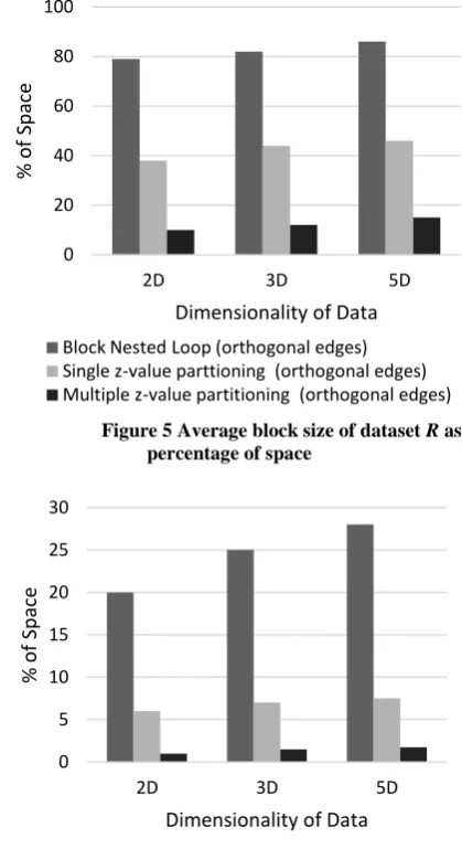
In Figure 3, the z-values values computed for the cells (4, 4) and (1, 5) will fix them next to each other in the sequential ordering of cells’ key values that does not reflect the actual Euclidean distance between the two cells. On the other hand the z-values Hilbert values computed for the cells (4, 4) and (1, 5) from a different starting point other than (1, 1) will not fix them next to each other in the sequential ordering of the cells’ key values that does not reflect the near proximity of the two cells. But the positions in the sequential order of the z-values of the cells (5, 5), (5, 6), (6, 5) and (6, 6) reflect their proximities. Hence the starting position for the computation of z2 must be chosen carefully that eliminates this anomaly. Subsequently, both z1 and z2 were used for partitioning the dataset into pre-determined set of partitions. The results of the experiments using controlled datasets are given in Figure 5 and in Figure 6 to prove the efficiency of this approach.

Figure 5 Average block size of dataset R as percentage of space

Figure 6 Average percentage difference in the block size of dataset S with respect to block size of R (in terms of

space)

The sizes of both datasets R and S was 100K each in terms of count of data elements. The number of partitions of dataset R was fixed at 50. Dimensions varied from two to five. The data belonged to unit space. The Voronoi based partitioning was ignored due to non-scalability of the method to higher dimensions and computational complexity. Figure 5 gives the Average Block Size (ABS) of dataset R as percentage of space. Since the data are randomly blocked in block nested loop method the ABS became uncontrollable and hence occupied very high percentage of space and the overlapping of these blocks were too many. The kind of discipline introduced by z-values resulted in reduction of the block sizes. The more number of z-values progressed towards optimal blocking. Figure 6 compares the difference in sizes of the blocks from R and S. The results show that the blocks of the datasets that are sent to the reducers tend to represent identical space.

0 20 40 60 80 100

2D 3D 5D

%

o

f

Sp

ace

Dimensionality of Data

Block Nested Loop (orthogonal edges) Single z-value parttioning (orthogonal edges) Multiple z-value partitioning (orthogonal edges)

0 5 10 15 20 25 30

2D 3D 5D

%

o

f

Sp

ace

Dimensionality of Data

4.

kNN

JOINS ON R*-TREES

The improved kNN join algorithm may be seamlessly extended to kNN join on two R*-Trees. Consider two R-Trees R and S. Based on the block handling capacities of the mappers, the partitioning can be done exploiting the hierarchical organization of the R-Trees. These partitions may them be fed into the reducers after properly shuffling the blocks created by the mappers. A brief description of the jobs done in each phase is given below.

Map Phase

In the map phase the leaf nodes of both the R-Trees R and S, on whom kNN join is required to be computed are grouped according to the block handling capacity of mappers. For effective grouping of the dataset two different z-values are computed for every data point if not already done during the construction of R-Tree. A regular sifting between the nodes and their parents is done for determining the best nearest neighbors that would reduce the number of reducers.

Shuffling Phase

In this phase every block of R-Tree of R is combined with the appropriate block of R-Tree of S based in the key values generated in the Map phase. Each pair of blocks is supplied to a Reducer.

Reduce Phase

In this phase the Reducers perform the kNN join on the pairs of blocks given to them. Any baseline join algorithm may be applied to join the blocks. Efficiency may be achieved by using sorting and searching algorithms on the datasets.

5.

EXPERIMENTAL SETUP AND

RESULTS

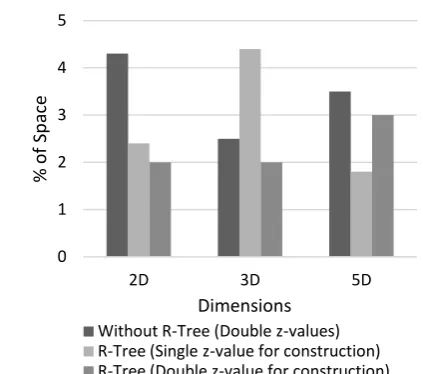
For the sake of conducting the experiments the same dataset that was discussed earlier was used. The number of partitions was kept at 50. Initially the kNN join was performed on the dataset without constructing an R-Tree. Double z-values were used for partitioning. After that the R*-Trees were constructed for both R and S datasets using single z-value. Later in the Map phase, double z-values were used for partitioning. The kNN join was performed on the constructed R*-Trees. Once again, the R*-Trees were constructed for both R and S datasets using double z-value. The kNN join was performed on the constructed R*-Trees. The results are presented in Figure 7 and Figure 8. The parameters that were measured in the experimental result presented in section 3 were measured for this experiment also. The results show that the consideration of more z-values resulted in better kNN join on two different multidimensional datasets.

Figure 7 Average block size of partitions of R and S in

terms of percentage of space

Figure 8 Average percentage difference in the block size of dataset S with respect to block size of R

(in terms of space)

6.

CONCLUSION

This paper proposed an improvement to the kNN join methods in a distributed environment, specifically Hadoop and Mapreduce. The proposed method uses multiple z-values for enhancing the performance on kNN joins. The paper also presented the adaptation of the multiple z-value strategy for applying kNN join on two R-Trees. The experimental results bear testimonial for the effectiveness of the amendments proposed.

7.

REFERENCES

[1] Jeffrey Dean and Sanjay Ghemawat, 2004, "Mapreduce: simplified data processing on large clusters", Proceedings of the 6th Conference on Symposium on Operating Systems Design & Implementation, vol. 6.

[2] Guttman, 1984, "R-trees: A dynamic index structure for spatial searching," Proceedings of the ACM SIGMOD International Conference on Management of

0 2 4 6 8 10 12 14

2D 3D 5D

%

o

f

Sp

ace

Dimensions

Without R-Tree (Double z-values) R-Tree (Single z-value for construction) R-Tree (Double z-values for construction)

0 1 2 3 4 5

2D 3D 5D

%

o

f

Sp

ace

Dimensions

[3] N. Beckmann, H. -P. Krieger, R. Schneider and B. Seeger, 1990, “The R*-tree: an efficient and robust access method for points and rectangles," Proceedings of the ACM SIGMOD International Conference on Management of Data, pp. 322-331.

[4] V. Gaede and 0. Guenther, 1998, "Multidimensional access methods," ACM Computing Surveys, vol. 30, no. 2, pp. 170-231.

[5] Y. Manolopoulos, A. Nanopoulos, A. N. Papadopoulos and Y. Theodoridis, 2003, “R-trees have grown everywhere," Technical Report, Available at http://citeseer.ist.psu.edu/706599.html.

[6] S. Brakatsoulas, D. Pfoser and Y. Theodoridis, 2002, "Revisiting R-tree construction principles," Proceedings of the 6th ADBIS Conference, pp. 149-162.

[7] L. Chen, R. Choubey and E. A. Rundensteiner, 1998, "Bulk-insertions into R-trees using the small-tree-large-tree approach," Proceedings of the 6th ACM GIS Conference, pp. 161-162.

[8] Daniar Achakeev, Marc Seidemann, Markus Schmidt and Bernhard Seeger, 2012, “Sort-based parallel loading of R-trees,” Proceedings of the 1st ACM SIGSPATIAL International Workshop on Analytics for Big Geospatial Data, pp. 62-70.

[9] Faloutsos and I. Kamel, 1994, "Beyond uniformity and independence: Analysis of R-trees using the concept of fractal dimension," Proceedings of the 13th ACMPODS Conference, pp. 4-13.

[10]I. Kamel and C. Faloutsos, 1994, "Hilbert R-tree: An improved R-tree using fractals," Proceedings of the 20th International Conference on Very Large Databases, pp. 500-509.

[11]F. Sagayaraj Francis and P. Xavier, 2014, "Amendments to the R*-Tree Construction Principles in Distributed Environment", International Journal of Engineering Research & Technology, vol. 3, Issue 5.

[12]Christos Doulkeridis and Kjetil Norvag, 2013, “A Survey of Large-Scale Analytical Query Processing in Mapreduce,” The VLDB Journal, DOI: 10.1007/s00778-013-0319-9.

[13]Himanshu Gupta, Bhupesh Chawda, Sumit Negi, Tanveer A. Faruquie, L. V. Subramaniam and Mukesh Mohania, 2013, “Processing multi-way spatial joins on map-reduce,” Proceedings of the 16th International Conference on Extending Database Technology, pp. 113-124.

[14]Afrati, F.N. and Ullman, J.D., 2010, “Optimizing Joins in a Map-Reduce Environment”, Proceedings of the 13th International Conference on Extending Database Technology, pp. 99–110.

[15]Nodarakis, N.; Pitoura, E.; Sioutas, S.; Tsakalidis, A.; Tsoumakos, D.; and Tzimas, G., 2014, “Efficient Multidimensional AkNN Query Processing in the Cloud”, Proceeding of the 25th International Conference on Database and Expert Systems Applications, pp. 1016-1027.

[16]Lu, W., Shen, Y., Chen, S. and Ooi, B.C., 2012, “Efficient Processing of k Nearest Neighbor Joins using Mapreduce”, Proceedings of the VLDB Endowment, vol. 5, Issue 10.