Robust Real Time Stereoscopic Alignment

Robust Real-Time Stereoscopic Alignment

Ross S Davies

University of South Wales School of Computing and Mathematical Sciences

CF37 1DL

Ian David Wilson

University of South Wales School of Computing and Mathematical Sciences

CF37 1DL

Andrew Ware

University of South Wales School of Computing and Mathematical Sciences

CF37 1DL

ABS TRACT

This paper presents a method for non-computationally expensive automatic alignment of cameras that utilises stereoscopic imagery separated at varying distances just below that of the intraocular distance. Here, automatic stereoscopic alignment in real-time is a non-trivial process that relies on calculating the best virtual alignment of camera lenses through image overlaying. This is important as retail 3D camera lenses are typically not sufficiently calibrated for accurate estimates of distance. The alignment of images allows the filtering of background objects and focuses on points of interest. Imprecision in camera lens calibration leads to problems with the required alignment of images and consequent filtering of background objects. The algorithm presented in this paper allows virtual calibration within non-calibrated cameras to provide a real-time filtering of images and the consequent identification of points of interest. The proposed method is capable of generating the best alignment setup at a reasonable computational expense in natural environments with partial background occlusion.

General Terms

KEYWORDS

Computer vision, Stereoscopic calibration, Stereoscopic vision

1

INTRODUCTION

Computer vision is a challenging field of computing where the ability of an algorithm to produce a valid output is often not the only measure of success. Often, one of the biggest problems in computer vision is the computation cost to run the algorithm in real-time.

In the field of computer vision, numerous algorithms have been created that have potential to solve a specific problem. For example, in previous work by the authors, a stereoscopic comparison algorithm has been developed to provide a partial solution to the human detection part of the vision problem [1]. Although a significant step forward, the application of this new algorithm is constrained by stereoscopic cameras suffering from a lack of calibration. Here, cameras of the same make and model do not necessarily work when put directly into the algorithm due to slight differences in lens alignments. In this paper, a solution for the problem is presented using part of the previous system’s comparison method.

The problem of different physical alignments on alternate cameras is not the only issue solved with this solution. Through aligning the image with different values, the ability to focus on different distance objects is possible. However, this requires compensation for the lack of physical lens alignment, which is here implemented virtually to provide a means for automatic alignment of images retrieved from each lens. This automatic alignment is essential for the successful

application of the human detection algorithm in both far and near environments.

Throughout this paper, all statistics are reported from tests performed on a computer running Windows XP, with access to a single 3.4 GHz core processor, 1GB memory (370MB used by OS). It is a clean operating system only running typical background processes such as anti-virus. This provides a fair and stable testing environment. The camera used is a stereoscopic camera recording at VGA resolution (640x480) at 60 fps (frames per second).

2

BACKGROUND AND MOTIVATION

Accurate human recognition is a significant computer vision problem, one to which a number of possible solutions have been devised [2] [3] [4] [5] [6] [7]. These systems typically make use of offline processing, the ones that do not have limited scope of use, which is discussed in the following section.

Algorithms such as Pfinder (“people finder”) [2] record multiple frames of unoccupied background taking one or more seconds to generate a background model. This model is subtracted from an image before processing occurs. After background subtraction, the only details remaining are the “moving objects” which under most conditions should be people moving through the scene.. Pfinder has limitations in its ability to deal with scene movement. The scene is expected to be significantly less dynamic than the user meaning that if other objects move such as trees blowing in the wind the algorithm will fail.

researchers in the past use single lens cameras but this does not then provide them with the benefit of depth perception Another approach that has emerged in computer vision is utilising multiple different cameras provide various viewpoints of a scene. Stereoscopic systems such as [6] provide the ability for human tracking in natural environments. This system uses conventional difference checking techniques to determine where motion has occurred in a scene. Motion of both cameras combined generates a location of a human, including their limbs within a scene. This project produced a robust system capable of tracking multiple people with the limitation of the environment requiring pre-setup.

Multi-lens imagery when set up correctly can have more than the advantage of viewing different viewpoints. Two cameras set-up at a distance close to that of the intraocular distance facing towards the same focal-point provides for stereoscopic imagery with the ability to extract a perception of depth. Finding out the displacement between matching pixels in the two images allows creation of a disparity map. This includes the depth information for each pixel viewable by both cameras. It is possible to extract and reconstruct 3-D surfaces from the depth map [8] [9]. Work conducted into depth mapping has improved the clarity of the result [10]. In [11], disparity estimation was improved by repairing occlusion. This allows for a more realistic depth map as occluded pixels are approximated from surrounding data. Processing requirements remains the fundamental problem that needs to be addressed for successful application in dynamic space in real-time. Generation of depth maps for the entire image is not currently possible in real-time. Research directed into subtracting regions out of an image using different techniques to give a smaller image to use for depth map generation. In previous work on stereoscopic human tracking, there has been multiple cameras set-up around an environment to gather information from different angles. There is a large amount of information held in just a short distance between cameras, evidenced in the subtraction stereo algorithm [12]. Using conventional techniques for background subtraction on both the right and left image, only the regions of “movement” remain. It is possible to generate a disparity map for only the relevant section of the image instead of the whole image when comparing movement in both images. The disparity then allows the extraction of data such as size and location of the object detected, which is not available in single view cameras. Although this is an improvement on single vision, the original proposed algorithm also extracted shadows [13]. In detection of pedestrians using subtraction stereo [7], the algorithm was expanded to exclude shadow information and a test case was put forward for the use of this algorithm in video surveillance. A further expansion of this work provided a robust system for tracking motion of individual persons between frames [13]. Camera calibration accounts for a large set of intrinsic parameters than alignment. Currently there are two methods of achieving this photogrammetric calibration which requires a reference object to allow the camera to see how it is interpreting the view [14] and self-calibration that traditionally can only be used in a static scene causing limitations for practical use. Even the most advanced self-calibration techniques require training within the scene and suffer from high computation. In [15] the authors created a calibration system that worked on the premise that the rotation point of a camera is not the optical centre. However, the system created is an accurate calibration method that suffers

the same as other methods in that it requires high computation due to the number of mathematical operations involved. Many of the parameters in stereoscopic vision calibration are not always required, especially in commercial applications replaced with a vital parameter of horizontal and vertical alignment. The alignment of the two cameras dictates the focal length of a stereoscopic system. Augmented Reality is a field of computing highly reliant on real-time computer vision where there are multiple users all with different mobile devices with a diverse set of camera types. In order to achieve high-speed robust vision based algorithms are required that work with a reduced set of calibration parameters. In [16] the errors introduced by a camera being able to move relative to the calibration frame were analysed. In the work produced the use of a stereoscopic camera reduces these errors as both cameras are subject to the same movements, hence making a large proportion of the alignment process unnecessary. The work here focuses on the parameter that has the most pull in stereoscopic systems the stereo-pair alignment. In previous systems, this value is treated as a fixed figure to calibrate the cameras for the optimum distance where the largest range of disparities are available. However, in our system this parameter is flexible based upon the premise of there being a specific transferrable region of interest in focus and the rest of the image needs to be considered noise. The alignment algorithm will adjust the parameter to filter out the background leaving the foreground disparities intact.

3

THE SYSTEM

The authors’ system previously presented [1] uses stereoscopic imagery separated at a distance just below that of the intraocular distance. The alignment of the images occurs manually through user interaction so that the objects in the distance appeared relative to each other in both images. A situation where the "line of sight" of both cameras is focused on background objects allowing an optimum representation to be formed.

(1)

h is the height of the input images. w is the width of the input images. y is the current row being evaluated. x is the current column being evaluated. left is the left camera lens input image. right is the right camera lens input image.

Figure 1: Valid Neighbours

(2)

A is a set of all pixels B = {A|A is a neighbour} h is the height of the image w is the width of the image y is the current row being evaluated. x is the current column being evaluated. t is the threshold

image is the output result from the difference filter

The evaluation function is comprised of equation one followed by equation two. The returned value is the count of valid pixels from two. Therefore, the absolute maximum is h multiplied by w and the minimum is zero.

Through this process, a representation of parallax is formed. The knowledge that closer objects have greater parallax than distant objects allows filtering of the resultant image to find the closest object without a prohibitive computational expense.

Table 1. Calculating the best threshold

Image

Lo

we

r

Th

re

sh

Upp

er

Th

re

sh

Arms open 105 110 Wall coloured top (low contrast) 109 174 Dark top (high contrast) 68 203 Close up 97 178 Distance (not closest / most prominent) 83 127 Distance (not closest / not prominent) 164 211 Average 104 167

Remaining pixels are separated into small regions representing portions of the image. These regions are clustered together to create larger regions of interest. The algorithm developed here runs on a set of images of size VGA (640 x 480) at 60fps. The algorithm without the alignment process is held back by the limitations of the capture device. Here, the alignment process does not infringe upon the systems functionality in real-time.

3.1

The Problem

The problem with this method is that the alignment values vary between different environments that include different distance backgrounds. Aligning this manually makes the algorithm flawed, as the whole point of computer vision is to allow the computer to work independently of human action. Analysis of a number of different scenes provides an alignment that works often with a given camera. However, the algorithm should also work on different cameras and be able to cope with varying background distances.

Alignment should not take place on just the horizontal axis. Even though the cameras are separated on the horizontal axis and should be aligned on the vertical axis this is not the case due to slight calibration problems with the camera. Required movement for alignment is smaller on the vertical axis than the horizontal.

3.2

Generating the Search Space

The image can be analysed and a single value assigned to the alignment. The best alignment returns the lowest value when most of the scene background is subtracted. The search space has global optima with a number of minor local optima. Although it is unlikely to fall into a local optimum, the possibility exists.

Images from both cameras are captured and converted to grey-scale, as at this stage speed is more important than the reduction in accuracy brought about by the use of a grey-scale. The images are aligned in the horizontal and vertical axis. The difference is calculated between each pixel in the images. At the next stage values that are considered as orphans are removed. Orphans are defined in the algorithm as a pixel that does not have a strong link, as determined by the threshold, to any of the horizontally or vertically connected pixels. When a link is present, the output value is incremented.

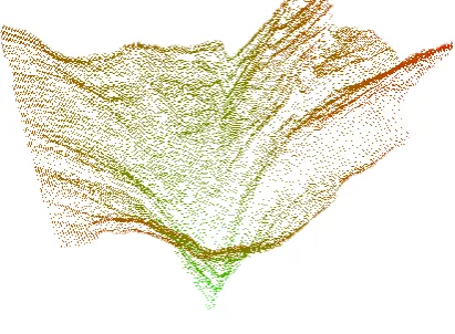
Figure 2: Typical search space

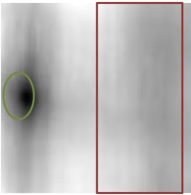
Figure 3: Raw image data

Figure 3 shows a top down view of the search space. Darker colours indicate a better match than lighter colours. This data has not been scaled and is the raw output from the algorithm that is indiscriminate of number of pixels. This means when the images are overlaid in a way that reduces the size of the final output, the value would naturally be less, as there is less available brightness in the image. So by scaling and finding a percentage of luminosity this problem is avoided. The larger white area in the middle is in-between the global (shown in green) and primary local optima (red shows the search space that leads away from the global optima).

Figure 4: Scaled image data

Leaving the data un-scaled produces a scenario that discriminates against close alignments. If two possible alignments exist, e.g. one close and one distant, without scaling the value to the number of pixels the distant one could possibly be a strong local optima causing a problem for the search process. However, by scaling the value relative to the amount of pixels in the alignment, distant alignments are no longer preferred. A comparison of the top of the images in the search space reveals this effect within the raw data. In Figure 3 the middle is made up of strong hill pushing values into the largest local optima. Although scaling does not remove the local optima, Figure 4 shows how the scope has been reduces.

Adding computation to an already slow process is not a desirable outcome. However, in this case it has proved to reduce the problem of a search space being potentially filled with minor local optima caused by image size variations. The tests below are in the range (-64) to (+64) in both the horizontal and vertical, this is a larger search space than would ever be required. Based upon work done to measure stereo camera depth accuracy it is known that cameras with a low separation distance (less than the intraocular) require less alignment and have a closer depth sensitivity [17]. Roughly, zero to 5% of the image size on the horizontal and ±2% on the vertical alignment would cover a wide range of medium resolution cameras with low separation distance. For VGA cameras this translates to a search space of (-10) to (+10) on the vertical axis and (0) to (30) on the horizontal axis. In comparison, scaling the data on the test alignment proved less resource hungry than anticipated, utilising 0.31 seconds extra processing capacity for an exhaustive search, which is an increase of approximately 3% of the overall computation expense.

Table 2. Raw and scaled search space comparison

Test Raw data Scaled data

1 10.673 10.979 2 10.761 11.044 3 10.736 11.061 4 10.746 11.034 5 10.692 11.044

Average 10.722 11.032

Std. Dev. 0.033 0.028

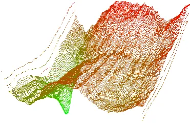
Figures 5 and 6 show the local optima produced when a person is in the scene during the alignment process. The global optimum is shadowed by how much search space drops into the local optima. Figure 5 shows the space before scaling the data. Noticeably the local optimum is far more evident and search methods have more chance of finding local rather than global optimum. This image is generated beyond the normal alignment constraints to show the possible extent of the problem.

Figure 6: Scaled local optima

Although Figure 6 shows that scaling does not solve the problem entirely, the significance of the local optima is minimal in comparison. Search methods have a greater chance of escaping these optima, as it is less prominent than the non-scaled version. It is important to note that this is a worst case scenario for the algorithm as a search space like this was only detected under certain lighting conditions with the person in question covering most of the background objects.

In a typical search space, generated local optima rarely occur in pictures where the alignment process is allowed to take place without a person present in the scene. Although being a realistic constraint it is impractical to try to avoid the possibility of local optima. The search methodology needs to be able to escape local optima. Metaheuristic techniques such as Simulated Annealing (SA) [18] and Tabu Search [19] are over complex and impose extra processing requirements. Instead, by analysing the results so far and the large extent of the global optima, a simpler solution, inspired by SA, was devised.

3.3

Original Solution

Normal hill climbing will be used when entering the algorithm based upon a best-fit starting alignment. When finding optima a new random starting position is generated, just as with SA. However, unlike SA, this new position will be analysed based on distance from the current best optima. The distance is measured using the Manhattan formula as diagonal moves are not valid steps so further precision is not required. Hill climbing is now run again and the best out of the two results will be returned. Due to the regularity of local optima in the search space, this search method is more than adequate to ensure the best possible alignment at a reasonable computational expense.

Algorithm:

1. Capture the left and right input images 2. Start at average best alignment position 3. Preform Hill Climbing to find optima 4. Save the match

5. Pick a random starting point

6. Preform Hill Climbing to find optima 7. Compare new match with previous result 8. Return best match

Hill climbing:

1. Evaluate position 2. Evaluate neighbours 3. Move to best neighbour 4. While improved go to 2 5. Return best match

Evaluate:

1. Using alignment preform difference filter 2. Remove orphan data

3. Count the remaining number of pixels

Here, alignment constraints were enforced as discussed earlier, the values were scaled and the test always started with the first pass hitting local optima. One hundred per cent of the passes under these conditions succeeded to find the global optima at significantly lower computational expense than an exhaustive search as shown in Table 3 and Table 4 where computational expense is measured in intervals. In all further tests, the global alignment was detected successfully where the background model was sufficiently visible. The largest portion of the image should be predominantly background rather than foreground objects.

Table 3. Exhaustive test images output

Test

Exhaustive Search

1 2 3 Average

1 1043 1052 1090 1061.67

2 1047 1046 1040 1044.33

3 1054 1073 1041 1056.00

Table 4. Algorithm test images output

Test

Algorithm

1 2 3 Average

1 118 77 115 103.33

2 83 82 97 87.33

3 117 80 86 94.33

3.4

Improved Solution

The previously proposed solution has one realistic constraint. One frame for the alignment process had to be taken in a vacant scene. This posed no problem upon system start-up but did cause problems if a subsequent calibration was required when the scene was occupied.

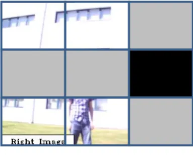
Figure 7: Split image

Algorithm:

1. Capture left and right input images 2. Start at average best alignment position 3. Preform Evaluation

4. Generate smaller images from worst region 5. Preform Hill Climbing to find optima 6. Save the match

7. Pick a random starting alignment 8. Preform Evaluation

9. Pick a region that is not on the same horizontal or vertical space on the grid.

10. Preform Hill Climbing to find optima 11. Final check (explained later)

12. Compare new match with

previous result 13. Return best match

Evaluation:

1. Preform difference filter 2. Preform orphan filter 3. Group data

4. Return lowest scoring region

Hill climbing:

1. Evaluate position 2. Evaluate neighbours 3. Move to best neighbour 4. While improved go to 2 5. Return best match

Evaluate:

1. Using alignment preform difference filter 2. Remove orphan data

3. Count the remaining number of pixels

Figure 7 shows how algorithm step nine works. The first region analysed is shown in black. The regions that are not valid for the next step of the analysis are shown in gray. The remaining four regions are valid for selection. The one that evaluates to the lowest out of these four is selected for further analysis.

Figure 8: Valid second regions

If the same result is generated as the first step then that value is returned. Otherwise, a final step is initialised (step 11 in the algorithm). In the worst cases were a local optima has been detected in either of the initial inputs, the selection process runs again. This time the new analysis cell is filtered out. In this Figure 9, it is shown with black, with horizontal and verticals shown in grey along with previously analysed or discounted regions. There is only one cell left for analysis. In most cases, this step will not be performed. It is only run if there is a small difference in the alignment values of a pixel or two, as the human would be assumed to be in focus in one of the regions.

Figure 9: Valid third regions

Although there are multiple extra steps in the improved algorithm, computationally it is less expensive. Only focusing on a small region in the image allows the evaluation function to preform quicker compensating for the extra steps. ComparingTable 5 and 4, it is evident that the algorithm not only works in a larger range of environments but also preforms alignment quicker.

Table 5. Improved algorithm test images output

Image

New

1 2 3 Average

20120305104735 71 66 59 60.33

20120305105249 84 59 76 71.00

4

CONCLUSION AND FURTHER

WORK

The solution provided here shows that the authors’ previous human detection algorithm through stereoscopic cameras has potential for utilisation outside of a preconfigured environment. The algorithm developed is robust against noise in the input images due to the orphan filter being performed after the initial alignment process. This filters out pixels that would otherwise be passed through from background noise or minor lighting errors. Only using one input frame from each of the input lenses taken almost simultaneously allows for the lighting independent alignment algorithm. Lighting changes will be the same in both the left and right footage as they are taken almost simultaneously

The alignment process was previously capable of preforming at 10fps. Improvements made on the algorithm increased the alignment on the same image to 16fps. That is a substantial increase in processing speed. However, the alignment process is only required when a significant change of environment is detected. For example, a significant change would be moving outdoors, indoors, to a different room or change in the focal distance of background. It is anticipated that large portions of the alignment computation will be moved to the graphical processing unit (GPU). For example, the difference check is a part of the algorithm that could move over to the GPU seamlessly resulting in a slight increase in the speed of the algorithm.

Higher resolution stereoscopic cameras potentially create an environment where local optimum exists in greater quantities with higher distribution throughout the search space. The solution proposed here works well with commercial stereoscopic webcams of both QVGA (320 x 240) to VGA quality. Further optimisation techniques may be necessary for higher resolution cameras, as a larger alignment search space would be required.

The previously proposed alignment algorithm required tests on both live and still images show that the alignment process works as expected when background is predominantly visible with only partial occlusion from foreground objects. A person can be visible in the scene as the algorithm is capable of releasing from local optima. However, it is preferable for the first frame of a scene to be unoccupied. This need to have an unoccupied scene is common in computer vision with popular techniques such as Pfinder [2] requiring relatively long initialisations of a second or more. Although there was nothing wrong with this requirement, it could potentially cause problems when alignment was necessary during runtime and the scene was occupied. The improved solution in this paper has provided liberation from this constrain with the algorithm being able to handle partial background occlusion. The alignment algorithm has proven to be successful allowing non-calibrated cameras to be utilised in real-time within a natural environment.

5

ACKNOWLEDGEMENT

This work is part-funded by the European Social Fund (ESF) through the European Union’s Convergence programme administered by the Welsh Government.

6

REFERENCES

[1] R. S. Davies, A. Ware and I. D. Wilson, “3D Human Detection,” 2013, Availiable from: http://intelligence.research.glam.ac.uk/documents/down

load/8

[2] C. R. Wren, A. Azarbayejani, T. Darrell and A. P. Pentland, “Pfinder: real-time tracking of the human body,” IEEE Transactions on Pattern Analysis and Machine Intelligence, vol. 19, no. 7, pp. 780 - 785, 1997.

[3] T. Bloom and A. P. Bradley, “Player Tracking and Stroke Recognition in Tennis Video,” in Proceedings of WDIC, 2003.

[4] K. Teachabarikiti, T. H. Chalidabhongse and A. Thammano, “Players Tracking and Ball Detection for an Automatic Tennis Video Annotation,” in 11th Int. Conf. Control, Automation, Robotics and Vision, Singapore, 2010.

[5] L. M. Fuentes and S. A. Velastin, “People tracking in surveillance applications,” Image and Vision Computing, vol. 24, p. 1165–1171, 2006.

[6] J. Amat, A. Casals and M. Frigola, “Stereoscopic System for Human Body Tracking in Natural Scenes,” in IEEE International Workshop on Modelling People MPeople99, Kerkyra , Greece, 1999.

[7] Y. Hashimoto, Y. Matsuki, T. Nakanishi, K. Umeda, K. Suzuki and Takashio, “Detection of pedestrians using subtraction stereo,” in International Symposium on Applications and the Internet, Turku , 2008 .

[8] R. Koch, “3-D surface reconstruction from stereoscopic image sequences,” in Fifth International Conference on Computer Vision, Cambridge, MA , USA , 1995.

[9] F. Devernay and 0. D. Faugeras, “Computing differential properties of 3-D shapes from stereoscopic images without 3-D models,” in Computer Society Conference on Computer Vision and Pattern Recognition , Seattle, WA , USA , 1994.

[10] L. Falkenhagen, “Depth Estimation from Stereoscopic Image Pairs Assuming Piecewise Continuos Surfaces,” Image Processing for Broadcast and Video Production, p. 115–127, 1994.

[11] W.-S. Jang and Y.-S. Ho, “Efficient Disparity Map Estimation Using Occlusion Handling for Various 3D Multimedia Applications,” IEEE Transactions on Consumer Electronics, vol. 57, no. 4, pp. 1937-1945, 2011.

[12] K. Umedaa, Y. Hashimotob, T. Nakanishib, K. Irieb and K. Terabayashia, “Subtraction stereo - A stereo camera system that focuses on moving regions,” in Three- Dimensional Imaging Metrology, San Jose, CA, USA, 2009.

[13] K. Terabayashi, Y. Hoshikawa, A. Moro and K. Umeda, “Improvement of Human Tracking in Stereoscopic Environment Using Subtraction Stereo with Shadow Detection,” International Journal of Automation Technology, vol. 5, no. 6, pp. 924-931, 2011.

and Machine Intelligence, vol. 22, no. 11, pp. 1330-1334, 2000.

[15] Q. Ji and S. Dai, “Self-Calibration of a Rotating Camera With a Translational Offset,” IEEE Transactions and robotics and automation, vol. 20, no. 1, Febuary 2004.

[16] E. Hayman and D. W. Murray, “The effects of translational misalignment in the self-calibration of rotating and zooming cameras,” IEEE Transactioins on Pattern Analysis and Machinie Intelligence, vol. 25, no. 8, pp. 1015-1020, August 2003.

[17] M. Kytö, M. Nuutinen and P. Oittinen, “Method for

mesuring stereo camera depth accuracy based on stereoscopic vision,” in Proc. SPIE 7864, 2011. [18] S. Kirkpatrick, C. D. Gelatt and M. P. Vecchi,

“Optimization by Simulated Annealing,” Science, vol. 220, no. 4598, pp. 671-680, 1983.