Inverse Rayleigh
Software Reliability Growth Model
B.Vara Prasad Rao
Associate Professor of Computer Science, Department of Computer Science & Engineering, R.V.R & J.C College of Engineering , Chowdavaram,Guntur- 522 019, Andhra Pradesh, India.
K.Gangadhara Rao
Associate Professor of Computer Science, Department of Computer Science & Engineering,Acharya Nagarjuna University, Guntur- 522 010, Andhra Pradesh, India.
B.Srinivasa Rao
Associate Professor of Statistics, Department of Mathematics & Humanities, R.V.R & J.C College of Engineering , Chowdavaram,
Guntur- 522 019, Andhra Pradesh, India.
ABSTRACT
A Non Homogenous Poisson Process (NHPP) with its mean value function generated by the cumulative distribution function of in-verse Rayleigh distribution is considered. It is modeled to as-sess the failure phenomenon of a developed software. When the failure data is in the form of number of failures in a given in-terval of time the model parameters are estimated by the max-imum likelihood method. The performance of the model using four data sets is discussed in comparison with existing models.
General Terms:
NHPP- non homogenous poisson process SRGM- software reliability growth model MLE- maximum likelihood estimation MSE- mean square error
IRD- inverse Rayleigh distribution
Keywords:
IRD,MLE,MSE,NHPP,SRGM
1. INTRODUCTION
It is well-known that computers are used in diverse areas for various applications. The growing importance of software dic-tates that a reliable software is by all means essential. A soft-ware itself does not fail unless the faults within the softsoft-ware re-sult in its failure. Generally, software faults are more difficult to handle. All design faults are present from the time the soft-ware is installed in the computer. A softsoft-ware fault inherent in a program is not dangerous unless and until it results in a failure of software. Accordingly, the concept of software reliability is rather dependent on the failure of a software and its frequency rather than the unknown number of faults latent in the software. Therefore, the term software reliability may be defined as the probability of failure free functioning of a software rather than the faults contained in it. However we cannot risk out the fact that software reliability depends on the number of faults also. In this regard, theory of probability and hence statistical anal-ysis have become essential in the development of a model that
can be used to evaluate the reliability of real world software sys-tems. Quantifying the software quality in terms of reliability is attempted through the study of software reliability growth mod-els.Software reliability models are statistical models which can be used to make predictions about a software system’s failure rate , given the failure history of the system. The models make assumptions about a fault discovery and removal process. These assumptions determine the form of the model and the meaning of the model’s parameters. Some recent works in this regard are by Akaike(1974) [1], Yamadaet al(1986) [15], Huanget al(1999) [10], Phamet al(1999) [13], Huanget al(2000) [11], Kapuret al(2002) [3], Haung and Kuo(2002) [6], Pham and Zhang(2003) [18], Yamadaet al(2003) [20], Yamada and In-oue(2004) [22], Huang(2005) [7], Huang and Lyu(2005) [8], Ka-puret al(2005) [2], Pham(2005) [5], Quadriet al(2006) [16], Huanget al(2007) [23], Lan and Leemis(2007) [12]. With this backdrop, we study the modeling of software reliability as a Non Homogenous Poisson Process (NHPP) with mean value function based on inverse Rayleigh distribution. Similar at-tempts based on Pareto distribution is made by Kantam and Sub-barao(2009) [9] and that based on half logistic distribution is given by Srinivasa Raoet al(2011) [19] .The genesis and the development of the model with the necessary input about a Non Homogenous Poisson Process are presented in Section 2. Max-imum likelihood (ML) estimation of the parameters of the de-veloped software reliability growth model (SRGM) is discussed in Section 3. The proposed SRGM is then compared with other software reliability growth models in Section 4. The concept of cost aspect in developing a software , associated randomness and the optimum release time of a developed software with respect to cost aspect are given in Section 5. Summary and Conclusions are given in Section 6.
2. SRGM AS A NON HOMOGENOUS POISSON
PROCESS
of events that have occurred in a specified interval of time. Let it be denoted byN(t), wheretis any non negative real number.
N(t)indicates the number of random occurrences in the interval
[0,t]. A counting process is said to be a Poisson process if the failure has stationary independent increments and the number of failures in any time interval of lengthshas a Poisson distribution with meanλsgiven by
P(N(t + s)−N(t) = y) =e
−λs(λs)y
y! ,y = 0,1,2, ... (1)
This mathematical model indicates that the changes inN(t)from one time period to another time period say[t,t+s]depend only on the length of the intervalsbut not on the extremitiest,t+sof the interval.λis called the failure intensity. In the above equation
E[N(t)] =λt,∀t. If we think of a Poisson process whose mean depends on the startingtand also the length of the intervalssuch a Poisson process can be explained by an equation as
P(N(t) = y) =e
−m(t)(m(t))y
y! ,y = 0,1,2, ... (2)
In this equationm(t)is a positive valued, non decreasing, contin-uous function oft, generally tending to a finite limit ’a’ ast→ ∞.m(t)is called the mean value function and its derivative with respect totis the intensity functionλ(t). Equation (2) is called a Non Homogenous Poisson Process. If a software system when put to use fails with probabilityF(t)before timet, if ’a’ stands for the unknown eventual number of failures that it is likely to experience, then the average number of failures expected to be experienced before timetisaF(t). HenceaF(t)can be taken as the mean value function of an NHPP. In the theory of probabil-ity,F(t)is called the cumulative distribution function (CDF) of a continuous non negative valued random variable. Thus an NHPP designed to study the failure process of a software can be con-structed as a Poisson process with mean value function based on the cumulative distribution function of a continuous positive valued random variable. Since a number of distributions is avail-able in statistical science, one can think of a number of NHPP models each based on a CDF. The first and foremost of such models is due to Goel and Okumoto(1979) [4] which is based on the well-known exponential distribution. Later many such mod-els have been suggested and studied by various researchers that can be found in Wood(1996) [21], Pham(2000) [17] and Huang
et al(2007) [23] and references therein. The probability density function (pdf)of inverse Rayleigh distribution (IRD)with scale parameter b is
f(x) = 2b x3e
(− b
x2), x >0, b >0 (3)
Its cumulative distribution function (cdf) is given by
F(x) =e(−xb2), x >0, b >0 (4)
We consider an NHPP with the mean value function given in terms of the CDF of inverse Rayleigh distribution(IRD) given as
m(t) = e−t2b ×a a>0,t>0 (5) It can be seen thatm(t)tends to ’a’ as t → ∞andm(t) is a positive valued non decreasing function oft.
The reliability in the software system with the above modeling is the probability of no failures in the time interval[0,t]and is given by
R(t) = P{N(t) = 0}= e−m(t) (6) In general, the reliabilityR(x/t)the probability that there are no failures in the interval[t,t+x]is given by
R(x/t) = P{N(t + x)−N(t) = 0}= e−[m(t+x)−m(t)] (7)
Generally, the expression given in Equation (7) is called software reliability based on NHPP and this is also called as software re-liability growth model (SRGM). If the mean value function is completely specified with its parameters we can have the value of the software reliability at any time of our choice. If the param-eters of the mean value function are not known they need to be estimated by a software failure data in the form of failure counts which can be used to get an estimate of the software reliability in order to assess the software quality. We present the ML es-timation of parameters in an NHPP based on inverse Rayleigh distribution in section 3.
3. ML ESTIMATION
Suppose that software failure data are given in the form of
(yi, ti)i=1,2,...n whereyiis the number of failures observed in
the interval[0, ti]i=1,2,...n with0< t1 < t2 < ... < tn. Such
a data is called failure count data. The log likelihood function to get the estimates of parameters of the NHPP shall be of the form
LLF = n X
i=1
(yi−yi−1)log[m(ti)−m(ti−1)]−m(tn) (8)
∂
∂a(LLF) = 0,⇒a = yn×e
b
t2n (9)
∂
∂b(LLF) = 0,⇒ n X
i=1 t2
i−1e −b t2
i−1 −t2
ie −b t2 i
e −b t2
i −e
−b t2
i−1
(yi−yi−1)−ynt2n= 0
Table 3.1
Data Set 1 Data Set 2 Data Set 3 Data Set 4
Test CPU defects CPU defects CPU defects CPU defects
Week hours found hours found hours found hours found
1 519 16 384 13 162 6 254 1
2 968 24 1186 18 499 9 788 3
3 1,430 27 1471 26 715 13 1054 8
4 1,893 33 2236 34 1137 20 1393 9
5 2,490 41 2772 40 1799 28 2216 11
6 3,058 49 2967 48 2438 40 2880 16
7 3,625 54 3812 61 2818 48 3593 19
8 4,422 58 4880 75 3574 54 4281 25
9 5,218 69 6104 84 4234 57 5180 27
10 5,823 75 6634 89 4680 59 6003 29
11 6,539 81 7229 95 4955 60 7621 32
12 7,083 86 8072 100 5053 61 8783 32
13 7,487 90 8484 104 — — 9604 36
14 7,846 93 8847 110 — — 10064 38
15 8,205 96 9253 112 — — 10560 39
16 8,564 98 9712 114 — — 11008 39
17 8,923 99 10083 117 — — 11237 41
18 9,282 100 10174 118 — — 11243 42
19 9,641 100 10272 120 — — 11305 42
20 10,000 100 — — — — — —
4. COMPARATIVE STUDY
The present SRGM based on NHPP model can be compared with other models also w.r.t some criteria of preference. The standard models that are considered here are those based on the
(i) Exponential cumulative distribution function. (ii) Half logistic cumulative distribution function.
(iii) Gamma cumulative distribution function with shape param-eter 2.
in succession. The first NHPP is called Goel -Okumoto model (1979) [4]. The second NHPP is software reliability growth model based on half logistic model(2011) [19]. The third NHPP is called Yamada S-shaped software reliability growth model (1983) [14]. For a ready reference,given below are the mean value functions and associated results of differentiation useful to get the ML estimates of the parameters in our proposed model and the three competitive models.
(1) Inverse Rayleigh Distribution(The proposed model):
n P
i=1 t2i−1e
−b t2
i−1−t2ie −b t2 i
e −b t2
i −e −b t2
i−1
(yi−yi−1) + ynt2n= 0
a = yn×e
b t2n
(2) Exponential Distribution(Goel-Okumoto(1979) [4] Model):
n P
i=1
tie−bti−ti−1e−bti−1
e−bti−1−e−bti (yi−yi−1)−yntne −btn
1−e−btn = 0
a = yn
1−e−btn
(3) Half Logistic Distribution:
n P
i=1
tie−bti (1+e−bti )2
− ti−1 e−bti−1 (1+e−bti−1 )2
ˆ
a[ −2e−bti (1+e−bti )(1−e−bti−1 )]
(yi−yi−1)− tne
−btn
(1+e−btn)2 = 0
a = yn× 1+e −btn
1−e−btn
(4) Gamma Distribution (Yamada(1983) [14] Model):
n P
i=1 t2
ie
−bti−t2 i−1e
−bti−1
ˆ
a[(1+bti−1)e−bti−1−(1−bti)e−bti]
(yi−yi−1)−at2ne−btn= 0 yn= a[1−(1 + btn)e−btn]
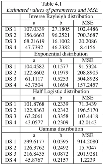
Now, we adopt calculation of mean square error(MSE) for model comparison. The formula is defined as
MSE =
n
P
i=1
(yi−m(ti))2
n−N where m(t)ˆ stands for MLE of
m(t). For four sets of Wood(1996), the MLE of the pa-rameters and the estimators of the mean value function are computed and thereby the values of MSE for various models. The results are given in the table 4.1.
Table 4.1
Estimated values of parameters and MSE
Inverse Rayleigh distribution
a b MSE
DS 1 107.0339 27.1805 102.4486
DS 2 156.6663 96.2521 700.3687
DS 3 68.21619 16.1002 20.2086
DS 4 47.7392 46.2382 8.4156
Exponential distribution
a b MSE
DS 1 104.4582 0.1577 91.5324
DS 2 122.8602 0.1979 208.8905
DS 3 61.1117 0.5253 504.8928
DS 4 43.7504 0.1694 157.2457
Half Logistic distribution
a b MSE
DS 1 101.8768 0.2339 71.3439
DS 2 122.8363 0.2342 196.5170
DS 3 63.2061 0.3358 103.4418
DS 4 43.0577 0.2309 42.0143
Gamma distribution
a b MSE
DS 1 299.6177 0.0595 914.2080
DS 2 126.3762 0.2492 15.7047
DS 3 216.8435 0.0872 201.9281
DS 4 45.8767 0.2157 1.2239
5. OPTIMAL RELEASE POLICY
[image:3.595.54.292.554.774.2]the testing time the more reliable the software is. However, the total cost of software development is also expected to increase. On the other hand, if the testing time is too short, though the cost of software development would be reduced we cannot avoid the customer’s risk of receiving unreliable software which in turn leads to increase in cost during the operational phase. Testing is an efficient way to remove faults in software products but testing of all possible executable paths in a general program is imprac-tical. To determine when to stop testing or when to release the software to customers keeping the expected total software cost at a minimum subject to warranty and risk is considered as an optimal release policy.
A cost model is essential to define important software cost fac-tors. It should help software developers in scheduling of re-sources for prompt delivery. Moreover with a reasonably suffi-cient reliability the model should contribute to decide an appro-priate release time of the software. With these objectives several software cost models are suggested (Pham(2000) [17],Chapter 6). In this section a software cost model with risk factor as dis-cussed in Pham(2000) [17] is adapted and the model is presented in the following lines for a ready reference. A software cost gen-erally consists of the following components.
(i) cost to perform testing
(ii) cost incurred in removing errors during testing phase
(iii) risk cost due to software failure.
Testing cost is denoted byC1t,wheretis the total test time.C1
is software test cost per unit time. IfN(t)stands for number of errors detected by timet, expected time to remove all these errors is given by
E N(t)
X
i=1 Yi
= E[N(t)]E[Yi] = m(t)µy (11)
whereYi is time to remove theitherror during testing phase,
m(t)is expected number of errors detected by timet,µyis
ex-pected time to remove an error during testing phase also called
E(Y). Therefore the expected cost to remove all errors is given byC2m(t)µywhereC2is cost of removing each error per unit
time during testing. The risk cost due to software failure, after releasing the software is
E(t) = C3[1−R(x/t)] (12)
whereC3 is cost due to software failure andR(x/t)is survival
probability of the software by xunits of time given it is tested fortunits of time.Therefore the total expected cost of software is given by
E(t) = C1t + C2m(t)µy+ C3[1−R(x/t)] (13)
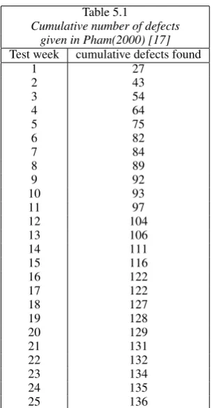
[image:4.595.353.505.93.386.2]The value oftthat minimizes the expected total cost in Equa-tion (13) is to be calculated. Such an optimal value of t is called optimal release time. In the expression form(t)in Equa-tion (13) is taken and the mean value function as given by IRD and t has to be solved. The formula for such a t has to be compared with the value of tfor a similar NHPP model say Goel & Okumoto(1979) [4], half logistic model (2011) [19] , Yamada(1983) [14] etc. The expected cost function given in equation(13) will show an increasing trend and falls down at a certain time and then increases from there. The time instant at which the change in the trend is observed is taken as the optimal time at which the testing is to be stopped and the product is ready for release . This methodology of locating optimum release time is explained with the data set given in Table 5.1.
Table 5.1
Cumulative number of defects given in Pham(2000) [17]
Test week cumulative defects found
1 27
2 43
3 54
4 64
5 75
6 82
7 84
8 89
9 92
10 93
11 97
12 104
13 106
14 111
15 116
16 122
17 122
18 127
19 128
20 129
21 131
22 132
23 134
24 135
25 136
For the above data , the parameteric values of IRD are a=136.8905 and b=13.2174. After estimating these values, the goodness of fit for 25 observations showed that R=0.8057. For the above data containing count of cumulative failures, let us start at an arbitrary choice of cumulative failures, say, let us note down the time by which 100 cumulative failures are ex-perienced. In the present example it is.. ”97 cumulative failures are observed within 11 weeks”. From that time onwards using the data on timeti, cumulative number of failuresyi, the
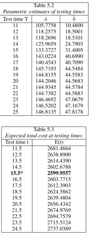
esti-mate of mean value function with the help of MLEs of the pa-rameters which are given in Table 5.2. is calculated . For the sake of explanation let us take the specified costsC1, C2, C3
asC1 = 25, C2 = 200, C3 = 7000,the choiceµybe kept at
µy= 0.1(as considered by Pham (2000) [17]). These
specifica-tions would help us to get the values of expected total software cost as given by Equation (13). For various times and cumulative failures of the data set, our chosen time is ”11thweek onwards”.
Therefore from 11th week onwards in the data set at each time pointE(t)can be calculated . These are given in Table 5.3 , which searches for a trend inE(t)from a rise to a fall and a rise after
11thweek onwards say 11.5 etc. It shows thatE(t)gives the
de-sired trend of rise-fall-rise at 15.5. Therefore, to release the soft-ware after15thweek before16thweek based on IRD is suggest.
The same data based on Goel-Okumoto model suggest to release after20thweek as worked out in Pham(2000) [17].Based on half
logistic model suggest to release after17thweek as worked out
Table 5.2
Parametric estimates of testing times
Test time T ˆa ˆb
11 105.7758 10.4800
12 118.2575 18.5001
13 118.2696 18.5101
14 125.9659 24.7903
15 133.3727 31.4005
16 143.0224 40.6990
17 140.4543 40.7090
18 145.7193 44.5484
19 144.8155 44.5583
20 144.2046 44.5683
21 144.9345 44.5784
22 144.7382 44.5883
23 146.4692 47.0679
24 146.5202 47.1679
25 146.8135 47.8178
Table 5.3
Expected total cost at testing times
Test time t E(t)
11.5 2681.4664
12.5 2638.8900
13.5 2614.4390
14.5 2602.6788
15.5* 2599.9557
16.5 2603.7715
17.5 2612.3903
18.5 2624.5862
19.5 2639.4804
20.5 2656.4342
21.5 2674.9769
22.5 2694.7579
23.5 2715.5124
24.5 2737.0389
6. CONCLUSIONS
The well known inverse Rayleigh distribution of the statistical science to develop a SRGM through NHPP is considered. Its suitability and preferability over three reliability growth mod-els is exemplified with the help of four live data sets . The delay in releasing a software product whose failure phenomenon is ap-proximated by our model, can be reduced in comparison with three competitive models Goel-Okumoto(1979) [4], half logistic (2011) [19] and Yamada(1983)[14].
Acknowledgments
The authors thank the editor and the reviewers for their helpful suggestions,comments and encouragement, which helped in im-proving the final version of the paper.
7. REFERENCES
[1] Akaike.H. A new look at statistical model identifica-tion. IEEE Transactions on Automatic Control, 19:716– 723, 1974.
[2] Anu Gupta. Kapur.P.K and Omphal Singh. On dis-crete software reliability growth model and categoriza-tion of faults. Operational Research Society of In-dia(OPSEARCH), 42(4):340–354, Dec 2005.
[3] Bardhan.A.K. Kapur.P.K. and Shatnawi.O. Why software reliability growth modelling should define errors of dif-ferent severity. Journal of Indian Statistical Association, 40(2):119–142, 2002.
[4] Goel.A.L. and Okumoto.K. A time dependent error de-tection rate model for software reliability and other per-formance measures. IEEE Transactions on Reliability, 28(3):206–211, 1979.
[5] Hoang Pham. A generalized logistic software reliabil-ity growth model. Operational Research Society of In-dia(OPSEARCH), 42(4):322–331, Dec 2005.
[6] Huang and Kuo.S.Y. Analysis of incorporating logistic test-ing effort function into software reliability modeltest-ing.IEEE Transactions on Reliability, 51(3):261–270, Sept 2002. [7] Huang.C.Y. Performance analysis of software reliability
growth models with testing-effort and change-point. Jour-nal of Systems and Software, 76(2), May 2005.
[8] Huang.C.Y. and Lyu.M.R. Optimal release time for soft-ware systems considering cost,testing-effort and test effi-ciency.IEEE transactions on Reliability, 54, Dec 2005. [9] Kantam.R.R.L. and Subba Rao.R. Pareto distribution - a
software reliability growth model.International Journal of Performability Engineering, 5(3):275–281, 2009.
[10] Kuo.S.Y. Huang.C.Y. and Lyu.M.R. Optimal software re-lease policy based on cost, reliability and testing efficiency. InProceedings of 23rd IEEE Annual International, 1999. [11] Kuo.S.Y. Huang.C.Y. and Lyu.M.R. Effort-index based
software reliability growth models and performance asses-ment. InProceedings of 24th IEEE Annual International Computer Software and Applications Conference, pages 454–459, 2000.
[12] Lan.Y. and Leemis.L. The logistic exponential survival dis-tribution.Naval Research Logistics, 55(3):252–264, 2007. [13] Nordmann.L. Pham.H. and Zhang.X. A general imperfect software debugging model with s-shaped fault detection rate.IEEE Transaction on Reliability, (48):169–175, 1999. [14] Ohba.M. Yamada.S. and Osaki.S. S-shaped reliability growth modeling for software error detection.IEEE Trans-actions on Reliability, 32(5):475–484, 1983.
[15] Ohtera.H. Yamada.S. and Narihisa.R. Software reliability growth models with testing effort. IEEE Transactions on Reliability, R-35:19–23, 1986.
[16] Peer.M.A. Quadri.S.M.K., Ahmad.N. and Kumar.M. Non-homogeneous poisson process software reliability growth model with generalized exponential testing effort function.
RAU Journal of Research, 16(1-2):159–163, 2006. [17] Pham.H.Software Reliability. Springer-Verlag, 2000. [18] Pham.H. and Zhang.X. Non homogeneous poisson process
software reliability and cost models with testing coverage.
European Journal of Operational Research, (145):443– 454, 2003.
[19] Srinivasa Rao.B., Vara Prasad Rao.B., Kantam.R.R.L., Software reliability growth model based on half logis-tic distribution. Journal of Testing and Evalaution, 39(6):1152–1157, 2011.
[20] Tamura.Y. Yamada.S. and Kimura.M. A software reli-ability growth model for a distributed development en-vironment. Electronic and Communications in Japan, 83(3):1446–1453, 2003.
[21] Wood.A.P. Predicting software reliability.IEEE Computer, 11:69–77, 1996.
[22] Yamada.S. and Inoue.S. Testing coverage dependent soft-ware reliability growth modeling. International Journal of Quality , Reliability and Safety Engineering, 11(4):303– 312, 2004.
[23] Yen.S.K. Huang.C.Y. and Michael.R.Lyu. An assesment of testing effort dependent software reliability growth models.