Analysing the Performance of Speaker Verification Task using Different Features

Analysing the performance of Speaker Verification

task using different features

L.Kavitha

Master of Engineering Department of CSE SSN College of Engineering, Chennai

B.Bharathi

Assistant Professor Department of CSE SSN College of Engineering, Chennai

ABSTRACT

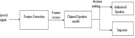
Speaker recognition is the identification of the person who is speaking by characteristics of their voices, also called “voice recognition”. The components of Speaker Recognition in-cludes Speaker Identification(SI) and Speaker Verification(SV). Speaker identification is the task of determining an unknown speakers identity. If the speaker claims to be of a certain iden-tity and the voice is to verify this claim, this is called Speaker Verification. It determines whether an unknown voice matches the known voice of a speaker whose identity is being claimed. This paper proposes Speaker Verification task. There are two phases in the Speaker Verification task namely, training and test-ing. In the training phase, different features such as Mel Fre-quency Cepstral Coefficient(MFCC), Linear Predictive Cepstral Coefficient(LPCC), Perceptual Linear Predictive(PLP) are ex-tracted from the speech signal and is trained by Support Vector Machine to get the target speaker model. It is trained with both actual speaker and impostor utterances. In the testing phase, fea-tures are extracted from the test speech signal . The test feafea-tures are extracted for different duration of time. The extracted feature vectors are given to the claimed speaker model and the decision is taken as authorised speaker or an impostor. The performance of a speaker verification task is analysed using different features with different utterance sizes. The result shows that the perfor-mance of a speaker verification task decreases when the duration of the speech utterances decreased.

General Terms:

Speaker Verification, Support Vector Machine

Keywords:

Mel Frequency Cepstral Coefficient(MFCC), Linear Predictive Cepstral Coefficient(LPCC), Perceptual Linear Predictive(PLP), Equal Error Rate(EER)

1. INTRODUCTION

Speech Processing extracts the information from a speech sig-nal. Speaker Recognition is the use of a machine to recognize a person from a spoken phrase. There are two modes of op-eration of these systems:to identify a particular person or to verify a person who claims for identity.In general for Speaker identification[1], there is no identity claim, and the system de-cides about who the person is, to what group the person is a mem-ber of, or that the person is unknown. It decides if the speaker is a specific person or among a group of persons. Speaker verifi-cation is defined as deciding if a speaker is whom he claims to

be, that is, a person makes an identity claim.Speaker verifica-tion is a popular biometric identificaverifica-tion technique used for au-thenticating and monitoring human subjects using their speech signal. The method is attractive for two reasons. It does not re-quire direct contact with the individual, thus avoiding the hurdle of perceived invasiveness inherent in many biometric systems. It does not require deployment of specialized signal transducers as microphones are now ubiquitous on most portable devices. Traditionally, speaker verification systems have been classified into two different categories based on the constraints imposed on the authentication process:

—Text-dependent speaker verification systems where the users are assumed to be cooperative and use identical pass-phrase during the training and testing phase.

—Text-independent speaker verification systems where no vo-cabulary constraints are imposed on the training and testing phase.

The operation of a speaker verification system[2] consists of two distinct phases:

—An enrollment phase where parameters of a speaker specific statistical model are determined using annotated (pre-labeled) speech data. It is the creation of a set of speech features, as a function of time for each valid user.

—A verification phase where an unknown speech sample is au-thenticated using the trained speaker specific model. It is the comparison of input speech with reference templates at equiv-alent points in time; decision based on similarity between the input and reference, integrated over time.

In both the phases the speech signal is first sampled, digitized and filtered before a feature extraction algorithm computes salient acoustic features from the speech signal. The next step in the enrollment phase uses the extracted features to train the speaker specific statistical model.

model. GMM uses a likelihood ratio for the conversion of variable data to fixed data. It is implemented by using the Universal Background Model. The alternate way to achieve a discriminative approach is by using Support Vector Machine. So we propose to implement the speaker verification using SVM.

2. PROPOSED METHOD

There are two phases in the proposed method:

Fig. 1. Training Phase in Proposed System

In training phase the following features are extracted from the input speech signal:

1. Mel Frequency Cepstral Coefficient(MFCC) 2. Linear Predictive Cepstral Coefficients(LPCC) 3. Perceptual Linear Predictive(PLP)

The extracted feature vectors are trained by Support Vector Ma-chine as the classifier. The training is done with both the actual speaker and the impostor utterances so as to obtain the target speaker model.

Fig. 2. Testing Phase in Proposed System

In testing phase different features are extracted from the test speech signal. These extracted feature vectors are given to the claimed speaker model. Here the obtained feature vectors are compared with actual feature vectors and the decision is taken for authorised speaker or impostor.

3. FEATURE EXTRACTION

The following features are extracted from the input speech signal

3.1 Mel Frequency Cepstral Coefficient

These are low level features which have been extensively used in speaker verification system. The key steps involved in computing MFCC [4] [2] features are:

(1) A sample of speech signal is first extracted using a window. Typically two parameters are important for the windowing procedure:

—the duration of the window which ranges from 20-30 ms and

—the shift between two consecutive windows which ranges from 10-15 ms.

The values correspond to the average duration for which the speech signal can be assumed to be stationary or its statis-tical and spectral information does not change significantly. The speech samples are then weighed by a suitable window-ing function, for example, Hammwindow-ing or Hannwindow-ing window are extensively used in speaker verification. The weighing reduces the artifacts (side lobe and signal leakage) of choos-ing a finite duration window size for analysis.

(2) The magnitude spectrum of the speech sample is then com-puted using a fast Fourier transform (FFT) and is then pro-cessed by a bank of band-pass filters. The filters that are generally used in MFCC computation are triangular filters, and their center frequencies are chosen according a logarith-mic frequency scale, which is also known as Mel-frequency scale.

(3) The filter bank is then used to transform the frequency bins to Mel-scale bins by the following equations:

my[b] =X f

wb[f]|Y[f]|2

where

—wb[f]is bth Mel-scale filters weight for the frequency f —Y[f]is FFT of the windowed speech signal

(4) The rationale for choosing a logarithmic frequency scale conforms to the response observed in human auditory sys-tems which has been validated through several biophysical experiments. The Mel-frequency weighted magnitude spec-trum is processed by a compressive non-linearity (typically a logarithmic function) which also models the observed re-sponse in a human auditory system.

(5) The last step in MFCC computation is a discrete cosine transform (DCT) which is used to de-correlate the Mel-scale filter outputs. A subset of the DCT coefficients is chosen (typically the first and the last few coefficients are ignored) and represent the MFCC features used in the enrollment and the verification phases.

Fig. 3. Steps involved in extraction of MFCC

3.2 Linear Predictive Cepstral Coefficient

At the core of the LPCC[2] feature extraction algorithm is the Linear Predictive Coding (LPC) technique which assumes that any speech signal can be modelled by a linear source-filter model. This model assumes two sources of human vocal sounds:

—Glottal pulse generator and —Random noise generator

In LPCC feature extraction[9], the filter is typically chosen to be an all-pole filter which is shown in fig. 4

The parameters of the all-pole filter are estimated using an

auto-Fig. 4. Steps involved in extraction of LPCC

regressive procedure where the signal at each time instant can be determined using a certain number of preceding samples.During an LPCC feature extraction, a quasi-stationary window of speech (about 20-30 ms) is used to determine the parameters ai and the process is repeated for the entire duration of the utterance. In most implementations, an overlapping window or a spectral shaping window is chosen to compensate for spectral degrada-tion due to finite window size. The estimadegrada-tion of the predic-tion coefficients ai is done by minimizing the predicpredic-tion error e(t). The prediction coefficients are then further transformed into Linear Predictive Cepstral Coefficients (LPCC) using a recursive method.

3.3 Perceptual Linear Predictive

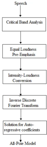
In PLP [5] [6] technique several properties of hearing are simu-lated by practical engineering approximations and the resulting auditorylike spectrum of speech is approximated by an autoag-gresive all-pole model.

The block diagram of PLP is shown in fig. 5

The key steps involved in computing PLP features are:

(1) The speech segment is weighted by the hamming window

W(n) = 0.54 + 0.46cos[ 2n

N−1] where N=length of the window.

The typical length of the window is about 20 ms. The Discrete Fourier Transform(DFT) transforms the windowed speech segment into the frequency domain. Typically Fast Fourier Transform(FFT) is used here. The real and imag-inary components of the short-term speech spectrum are squared and added to get the short-term power spectrum. (2) The spectrum is warped along its frequency axis into the

Bark Frequency and the resulting warped power spectrum is then convolved with the power spectrum of the simulated critical-band masking curve. This step is similar to spectral processing in mel cepstral analysis. The discrete convolu-tion yield samples of the critical-band power spectrum. The convolution with the relatively broad critical-band Masking curve significantly reduces the spectral resolution in com-parison with the original spectrum.

(3) The sampled interval is preemphasized by the simulated equal loudness curve.

(4) The last operation prior to the all-pole modelling is the cubic-root amplitude compression.This operation is an ap-proximation to the power law of hearing and simulates the nonlinear relation between the intensity of sound and its per-ceived loudness.

Fig. 5. Steps involved in extraction of PLP

(5) In the final operation of PLP analysis, amplitude compres-sion is approximated by the spectrum of an all-pole model using the auto-correlation method of all-pole spectral mod-elling. The inverse DFT(IDFT) is applied to yield the au-tocorrelation function.The IDFT is the better choice than the inverse FFT since only a few autocorrelation values are needed. The autoregressive coefficients obtained could be further transformed into some other set of parameters of in-terest, such as cepstral coefficients of the all-pole model.

4. SUPPORT VECTOR MACHINE

Support Vector Machines(SVMs)[7] [8] are an attractive choice for implementing discriminative models. SVMs are a set of re-lated supervised learning methods used for classification and regression. Support Vector Machine (SVM) is a classification and regression prediction tool that uses machine learning theory to maximize predictive accuracy while automatically avoiding over-fit to the data. SVMs were developed to solve the classi-fication problem, but now they have been extended to solve re-gression problems.

4.1 Margin

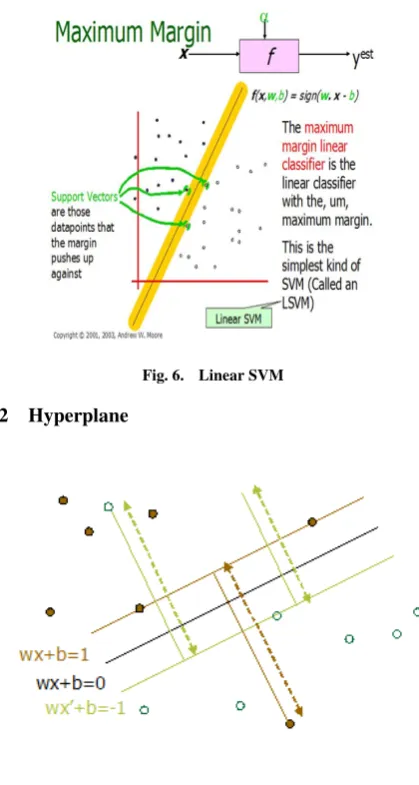
The above illustration is the maximum linear classifier with the maximum range. It is an example of a simple linear SVM classi-fier. The advantage is the better classification. The goals of SVM are separating the data with hyper plane and extend this to non-linear boundaries using a kernel trick.For calculating the SVM the goal is to correctly classify all the data. For mathematical calculations we have,

[a]If Yi= +1; wxi+b≥1 [b]If Yi=−1; wxi+b≤1

F or all i; yi(wi+b)≥1

Fig. 6. Linear SVM 4.2 Hyperplane

Fig. 7. Hyperplane

To separate the data should be greater than zero. From all pos-sible hyper planes [9], SVM selects one hyperplane where the distance is as large as possible. When the training data is good and every test vector is located in radius r from training vector and if the chosen hyper plane is located at the farthest possible from the data, the desired hyper plane which maximizes the mar-gin also bisects the lines between closest points on the convex hull of the two datasets. Distance of closest point on hyperplane to origin can be found by maximizing the x as x is on the hyper plane. This is given by

M aximumM argin=M = 2

||w||

4.3 Kernel

If data is linear, a separating hyper plane may be used to divide the data. If the data is far from linear and the datasets are in-separable, kernels are used for non-linear map the input data to a high-dimensional space. The mapping then results to linearly separable. An illustration is shown in the below figure:

The above mapping is defined by the Kernel:

K(x, y) = Φ(x).Φ(y) The different Kernel functions are listed below:

—Polynomial

—Gaussian Radial Basis Function

Fig. 8. Kernel —Exponential Radial Basis Function

4.3.1 Polynomial. A polynomial mapping is a popular method for nonlinear modeling. The second kernel is usually preferable as it avoids problems with the hessian becoming Zero.

K(x, x0_{) = (x, x}0₎d

K(x, x0) = ((x, x0) + 1)d where d is the degree of polynomial

4.3.2 Gaussian Radial Basis Function. Radial basis function is the most commonly used with a Gaussian form which is as follows

K(x, x0) =exp(−||x−x 0_||2

2σ2 )

where

σis Radial basis function

4.3.3 Exponential Radial Basis Function. A radial basis func-tion produces a piecewise linear solufunc-tion which can be attractive when discontinuities are acceptable.

K(x, x0) =exp(−||x−x 0_||

2σ2 )

where

σis Radial basis function

Radial Basis Function is used as the kernel type for this paper

5. EXPERIMENTAL SETUP

The dataset containing 50 speakers is used for all the experi-ments in this section.The speech corpus is created in a lab en-vironment with 50 speakers in which 43 are female speakers and 7 are male speakers and 142 utterances for each speaker with approximately of 3 seconds duration. The development set contains 100 utterances for training and 42 utterances for test-ing. In Training phase, the features such as MFCC, LPCC and PLP are extracted from the input speech signal. For MFCC, from each frame 39 coefficients are extracted which includes 13 Cep-stral coefficients, 13 acceleration coefficients and 13 delta coef-ficients. For LPCC, from each frame 12 Cepstral coefficients are extracted and for PLP, 13 coefficients are extracted from each frame. The extracted features are trained by Support Vector Ma-chine(SVM). The training is done with both actual speaker and impostor utterances so as to obtain the target speaker model. In Testing phase, the test features are extracted from the test speech signal. The test features extracted are of different dura-tion of time such as 3 Sec, 2 Sec, 1sec of time. The extracted features are given to the claimed speaker model. Here, the ob-tained feature vectors are compared with actual feature vectors and the decision is taken as authorised speaker or an impostor. If the result is authorised speaker, it is denoted by +1 and for im-poster it is denoted by -1.

6. PERFORMANCE EVALUATION

By analysing the features namely Mel Frequency Cepstral Co-efficient(MFCC), Linear Predictive Cepstral Coefficient(LPCC), Perceptual Linear Predictive(PLP) and its hybrid form PLP shows better performance.

The Equal Error Rate(EER) for each feature is shown in below tabulation

Table 1. Equal Error Rate for different features

EER MFCC LPCC PLP MFC+LPC MFC+PLP LPC+PLP

3sec 3.15% 3.29% 1.26% 6.70% 4.52% 2.68% 2sec 47.69% 47.62% 4.79% 48.50% 39.51% 42.01% 1sec 48.73% 48.23% 42.02% 49.00% 47.21% 47.94% 500ms 48.51% 48.79% 46.65% 48.09% 42.72% 48.99%

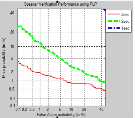
From table1 as the duration of time decreases, the Equal Error Rate increases thereby the performance decreases. It shows that among all the features PLP shows better performance for differ-ent duration of time. The performance is also shown in terms of the DET-curve

Fig. 9. Performance of Speaker verification task using PLP with different utterance size

From Fig. 9 as the duration of time decreases the Equal Error Rate increases and reaches beyond 40% which is not displayed in the graph.

7. CONCLUSION

In this paper, Speaker Verification using SVM, we propose to extract different features like Mel Frequency Cepstral Coef-ficient(MFCC), Linear Predictive Cepstral Coefficient(LPCC) and Perceptual Linear Predictive(PLP) for different utterance size(from 3s-500ms) and compared the performance of a speaker verification task. Among the features, PLP shows better per-formance in speaker verification task. The perper-formance of the speaker verification task can further be analysed by extracting discriminative features.

8. REFERENCES

[1] Ms. Arundhati S. Mehendale and Mrs. M. R. Dixit ”Speaker Identification”,An International journal in Sig-nal and Image Processing, Vol.2, June 2011.

[2] Amin Fazel and Shantanu Chakrabartty” An Overview of Statistical pattern Recognition Techniques for Speaker Ver-ification”. IEEE Circuits and Systems Magazine 2011. [3] Douglas A. Reynolds Thomas F. Quatieri and Robert B.

Dunn”Speaker Verification using Adapted Gaussian Mix-ture Models”,Digital Signal Processing, Vol.10, Nos. 1-3, January 2000

[4] Vibha Tiwari ”MFCC and its applications in Speaker recognition”,International Journal on Emerging Technolo-gies 1(1): 19-22(2010)

[5] Hynek Hermansky ”Perceptual Linear Predictive(PLP) analysis of Speech”, Journal of Acoustical Society of America, Vol.87, No.4:1738-1752 November 1989 [6] Petr Motlicek Vijay Ullal and Hynek Hermansky

”Wide-Band Perceptual Audio Coding based on Frequency-Domain Linear Prediction”, IEEE International Confer-ence on Acoustics, Speech and Signal Processing, Vol.1 I-265 - I-268, 2007

[7] Raghavan.S, G. Lazarou and J.Picone”Speaker Verifica-tion using Support Vector Machine”,IEEE Transaction on Computers, 2006

[8] Joseph P.Campbell”Speaker Verification: A tutorial”,Vol. 85, No.9 September 1997.