Paraconsistent Differential Calculus (Part II): Second Order Paraconsistent Derivative

(1)

http://dx.doi.org/10.4236/am.2014.58107

Paraconsistent Differential Calculus

(Part II): Second-Order Paraconsistent

Derivative

João Inácio Da Silva Filho

1,2

1_{Group of Applied Paraconsistent Logic, Santa Cecília University-UNISANTA, Santos, Brazil} 2_{Institute for Advanced Studies of the University of São Paulo-IEAUSP, São Paulo, Brazil}

Email: [email protected]

This work is licensed under the Creative Commons Attribution International License (CC BY). http://creativecommons.org/licenses/by/4.0/

Abstract

The Paraconsistent Logic (PL) is a non-classical logic and its main property is to present tolerance for contradiction in its fundamentals without the invalidation of the conclusions. In this paper, we use the PL in its annotated form, denominated Paraconsistent Annotated Logic with annotation of two values-PAL2v. This type of paraconsistent logic has an associated lattice that allows the de- velopment of a Paraconsistent Differential Calculus based on fundamentals and equations ob- tained by geometric interpretations. In this paper (Part II), it is presented a continuation of the first article (Part I) where the Paraconsistent Differential Calculus is given emphasis on the second-order Paraconsistent Derivative. We present some examples applying Paraconsistent De- rivatives at functions of first and second-order with the concepts of Paraconsistent Mathematics.

Keywords

Paraconsistent Logic, Paraconsistent Annotated Logic, Paraconsistent Mathematics, Paraconsistent Differential Calculus

1. Introduction

(2)

Paraconsistent Annotated Logic (PAL), there is in its representation an associated Lattice FOUR (Hasse Diagram) that allows the development of algorithmic techniques and direct applications, and that has brought promising results [2]-[4].

In this paper, we use the PAL in its structural form in which an annotation of two values is used to perform a type of Differential Paraconsistent Calculus applied in solving problem related to physical systems [5] [6]. The PAL treating information signals in its special form called Paraconsistent Logic with annotation of two values (PAL2v) allows to extract from the Newton’s quotient, found in the deduction of the differential calculus, all the information necessary and sufficient to effect the derivative of first and second order and apply them to physical systems with good results without ignoring the action of the infinitesimal.

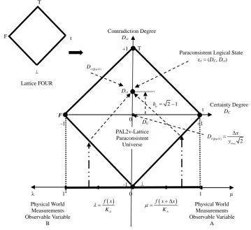
[image:2.595.132.492.377.706.2]

In the PAL2v-logic language an atomic proposition can be represented by P

(

µ λ,

)

, where μ and λ are ele- ments in the closed interval [0,1] what belongs to the set of real numbers. These two values are considered information signals and called by degrees of evidence. Among several intuitive readings, P

(

µ λ,

)

, can be read as: µ is the evidence favorable of the proposition P and λ the unfavorable evidence to proposition P. As seen in Figure 1in the associated Lattice, t and F represent the classical values true and False, respectively, and T de- notes Inconsistent, while⊥ Indetermination.Figure 1 shows the PAL2v-Lattice [4] [6].

In this representation, the PAL2v-lattice can be formed of ordered pairs of values

(

µ λ,

)

, which will form the annotation. In this representation, an operator ~ is fixed: τ →τ where: τ =

{

(

µ λ µ λ,

)

, ∈

[ ]

0,1

}

⊂R.

2. Paraconsistent Geometric Transformations

Paraconsistent Mathematics is structured on Paraconsistent Logic (PL) and has as main purpose the study of common mathematical objects such as sets, numbers and functions, where some contradictions are allowed. As proposed in [1] and in [4] it is possible through a lattice FOUR (Hasse Diagram) obtain in the PAL2v representation of how much the annotation (or evidences) can express the knowledge about a proposition P. It has been

T

F _t



Lattice FOUR

DC

Dct

λ 1 0 1 μ

F



T

t Certainty Degree _D_C

Contradiction Degree

Dct

-1 0 +1

+1 -1

Physical World Measurements Observable Variable

A Physical World

Measurements Observable Variable

B

Paraconsistent Logical State

ετ = (DC, Dct)

PAL2v-Lattice Paraconsistent

Universe

2 1

hψ= −

( ) ct Q N

D _ψ

( )

2

CQ N max

x D

y

ψ ∆ =

( ) ( )

N N

f x f x x

K K

λ= µ= + ∆

(3)

seen that through geometric transformations, we can find a PAL2v-Lattice τ of values, that it is equivalent to an associate Lattice FOUR. This form of interpretations allows Paraconsistent mathematical calculations through equations of parameterization. With Paraconsistent Geometric Transformation is considered the conversion of points in an Unitary Square on Cartesian Plane (USCP) in points into associative PAL2v-Lattice τ [3] [5] [7]. This final equation of Paraconsistent geometric Transformation is seen below:

(

_C, _ct

) (

, 1

)

T D D = µ λ µ λ− + − (1)

where: µ is favorable evidence degree assigned to the proposition P. λ favorable evidence degree assigned to the proposition P.

The first term of Paraconsistent Transformation is called the Certainty Degree (DC). Therefore, the Certainty

Degree is achieved by:

C

D = −µ λ (2)

Its values, which belong to the set ℜ vary in closed range −1 to +1 and are in the horizontal axis of the PAL2v-lattice τ of values called “Axis of degrees of certainty”.

The second term of Paraconsistent Transformation is called the Degree of Contradiction (Dct). Therefore, the

degree of contradiction is obtained by:

1

ct

D = + −µ λ (3)

The resulting values of Dct belong to set ℜ, vary on the closed interval +1 and −1 and are exposed on the ver-

tical axis of the PAL2v-lattice τ called “Axis of contradiction degrees”.

In the PAL2v-lattice τ when DC results in +1 it means that the Paraconsistent logical State (ετ) resulting from

the paraconsistent analysis is True, and when DC results in −1 it means that the Paraconsistent logical State (ετ)

resulting from the paraconsistent analysis is False. Similarly, in the PAL2v-lattice τ when Dct results in +1

means that the Paraconsistent logical State (ετ) resulting from the paraconsistent analysis is Inconsistent T, and when Dct result in −1 means that the Paraconsistent logical State (ετ) resulting from the paraconsistent analysis is

Undetermined ⊥. It is considered, therefore, that by analyzing the PAL2v-lattice τ [3] [6] the concept of Para- consistent logical State (ετ) can be correlated to the fundamental concept of state, as studied in physical science and then extended to the model based on Paraconsistent Logic. Therefore, the Paraconsistent logical State is represented by:

( , )

(

D DC, ct

)

τ µ λ

ε

= (4)

where: ετ is the Paraconsistent Logical state.

DC is the Certainty Degree obtained according to the two degrees of Evidence μ and λ.

Dct is the Contradiction Degree found according to the two degrees of Evidence μ and λ.

The Certainty Degree normalized from the Paraconsistent Logical Model is called Resulting Degree of Evi- dence which is calculated by:

Re

1 2

C D

µ = + (5)

Likewise, the normalized Contradiction Degree from the Paraconsistent Logical Model is calculated by:

1 2

Ct ctr

D

µ = + (6)

Derivative and Newton’s Quotient

In Calculus for the resolutions of problems of Physics the Derivative represents the instantaneous variation of a function [8]. If a function f is derivable or differentiable so close to each a point of its domain the function

( )

f x − f a will behave approximately as a linear function, so its graph is approximately a straight line [9] [10]. If the a point belongs to the interval, it is said that f is derivable in a if the limit exist and if it is finite. If this is the case, then this limit is called a Derivative of function f in the point a, and is represented by f′

( )

a

were:

( )

lim

( )

x a

f x f a f a

x a

→

−

′ =

(4)

Derivative can be rewritten as:

( )

(

)

( )

0

lim h

f a h f a f a

h

→

+ −

′ = . Likewise, the equation can be written as h

represents a variation of x, such that:

(

)

( )

0 0

lim lim

x x

f x x f x

y

x x

∆ → ∆ →

+ ∆ −

∆ ₌

∆ ∆ where Newton’s quotient is:

(

,

)

f x

(

x

)

f x

( )

Q y x

x + ∆ − ∆ =

∆ (7) Therefore, the Newton’s quotient is defined as the incremental ratio of f with respect to the variable x, at the point x [9] [11].

3. Paraconsistent Mathematics

The Newton’s quotient can adapt to a Paraconsistent Logical Model in the form of Paraconsistent mathematical Model will be formed based on the initial concepts of the derivatives [12] [13]. We will apply to the Newton’s quotient a K factor of normalization that aims to put its values within the limits of the PAL2v-lattice, therefore:

(

)

1

(

)

( )

, f x x f x

Q y x

x K K

+ ∆

 

∆ = _ − _

∆   (8) where: K is a normalization factor, whose action allows thee quation to be done as the fundamentals of PAL2v.

With the normalization factor in Equation (10) are identified Degrees of Evidence of PAL2v annotation, such

that: f x

(

x

)

K

µ

= + ∆ → Favorable Evidence Degree and f x

( )

K

λ

= → Unfavorable Evidence Degree.

From Equation (2) we have the Certainty Degree of the Newton’s quotient:

( )

(

)

( )

C N

f x x f x

D

K K

+ ∆

 

=_ − _

  (9) Similarly, from the Equation (3) the Contradiction Degree of the Newton’s quotient:

( )

(

) ( )

1

ct N

f x x x

D

K K

ψ

+ ∆

 

=_ + − _

  (10) In Paraconsistent Logic Model the K value must be estimated so that the values of the degrees of evidence become established with in the fundamentals of PAL2v. For this becomes: K ≥ f x

( )

This value can be an equilibrium constant equivalent to Planck’s constant called Paraquantum Factor of Quantization, as seen in [6].

max

2 N

K = y (11)

where: y_max the maximum value of the function at the considered point. KN Paraconsistent Newton Normalization Factor.

The value of the first-order Paraconsistent Derivative in the physical worldis obtained through reapplying the Newton Normalization Factor (KN) in the result of the in the Paraconsistent Newton’s quotient:

( )

N N

y′ =K ×PQ _ψ (12)

Thus, the Paraconsistent values extracted from Newton’s quotient adjusted to Paraconsistent Logical Model depend of ∆x, that is, the increment of the variable x applied to the calculations.

3.1. First-Order Paraconsistent Derivative

For a function of the type n

y=x where n is some positive integer, we have:

(

) ( )

0 0

lim lim

n n

x x

x x x

y

x x

∆ → ∆ →

+ ∆ −

∆ ₌

∆ ∆ .

(5)

sis will be written as:

( )

(

)

( )

n n

N

N N

x x x

PQ

K x K x

ψ

 _{+ ∆} 

= − 

∆ ∆

 

 

(13)

This normalization allows the function _y₌_xn_{to be identified in the Paraconsistent Newton’s quotient}_the Evidence Degree of a Paraconsistent Logical Model, such that:

(

)

n

N

x x

K ψ

µ = + ∆ → Favorable Evidence Degree and

( )

n

N N x

K ψ

λ = → Unfavorable Evidence Degree

The value corresponding to the Certainty Degree (DC) of the Paraconsistent Newton’s quotient, which, as the

fundamentals of PAL2v is obtained by Equation (9):

( )

(

) ( )

n n

C N

N N

x x x

D

K K

ψ

 _{+ ∆} 

= − 

 

 

(14)

Similarly, the Equation (10) the Contradiction Degree of the Paraconsistent Newton’s quotient:

( )

(

) ( )

1

n n

ct N

N N

x x x

D

K K

ψ

 _{+ ∆} 

= + − 

 

 

(15)

The Evidence Degree resulting Paraconsistent Newton’s quotient is:

( )

(

)

( )

Re

1

2 2 2

n n

Q N

N N

x x x

K K

ψ

µ = + ∆ − + (16)

And from the Equation (6) the normalized Contradiction Degree of Paraconsistent Newton’s quotient is:

( )

(

)

( )

2 2

N

n n

ctrQ

N N

x x x

K K

ψ

µ = + ∆ + (17)

3.2. Application Example

For example, if it is wished a final value of the first-order Paraconsistent Derivative of the function f x

( )

=x2

in x=5 so that the Contradiction Degree establishes thus a Paraconsistent Logical State ε of equilibrium of the PAL2v-Lattice τ.

Resolution: Initially, to form Paraconsistent Newton Normalization Factor it is calculated the maximum value of the function f x

( )

=x2 at the point considered x=5, therefore, being:

( )

2

( )

2

max 5 25

f x =x → f x =y → f x = =

It is calculated the value of the Paraconsistent Newton Normalization Factor, according to the Equation (12):

max

2 25 2

N N

K = y →K =

For an increment value of the variable x, for example, ∆ =x 0.001, Certainty Degree of Paraconsistent New- ton’s quotient is calculated by Equation (14):

( )

(

)

( )

2 2

5 0.001 5

0.00028287

25 2 25 2

CQ N CQ N

D _ψ = + − →D _ψ =

The Paraconsistent Newton’s quotient is calculated according to Equation (13):

( )

(

) ( )

( )

(

)

( )

[

]

( )

2 2 2 2

5 0.001 5

1 1

0.001 25 2 25 2

1

0.707389652 0.707106781 0.282870812

0.001

N N

x x x

PQ PQ

x K K

PQ PQ

ψ ψ

 _{+ ∆}   ₊ 

=  − → =  − 

∆ _ _ _ _

(6)

Recovering value of Paraconsistent Derivative in the physical world by Equation (12):

( ) 25 2 0.282870812 10.00993

N N

y′=K ×PQ_ψ → =y′ × =

Then, the value of the first-order Paraconsistent Derivative of the function f x

( )

=x2 at x=5 is: 10.00993

y′ = .

3.3. Paraconsistent Second-Order Derivative

Whereas the Paraconsistent Derivative of the first-order is obtained with the calculation of the Paraconsistent Newton’s quotient Equation (8), then the Certainty Degree is:

( )

(

)

( )

C Q N

N N

f x x f x

D

K K

ψ

+ ∆

 

=_ − _

  (18)

This first value of the Certainty Degree will be normalized by application Equation (5), turning into Evidence Favorable Degree to the second-order Derivative, so:

( ) 1 ( )

2

1

2 C Q N Q N

D _ψ

ψ

µ = + (19)

Or then, (18) in (19), resulting:

( )

(

)

( )

2

1

2

N N

Q N

f x x f x

K K

ψ µ

+ ∆

 

− +

 

 

= (20)

For second-order Paraconsistent Derivative representation, when the value of ∆x decreases will be the Un- favorable Evidence Degree (λ) to approach the Favorable Evidence Degree (µ). Therefore, the equation of pa- raconsistent Newton’s quotient of the second point, or second Paraconsistent Logical State, obtained into PAL2v- Lattice τ for second-order derivative is:

( )2

( )

(

)

1 N

N N

f x f x x

PQ

x K K

ψ

− ∆

 

=  − 

∆   (21) Are identified in the Equation (21) the degrees of evidence:

( )

2

N f x

K ψ

µ = → Second Favorable Evidence Degree.

(

)

2

N f x x

K ψ

λ = − ∆ → Second Unfavorable Evidence Degree.

Thus, in Paraconsistent Logical Model has been the Certainty Degree of second Logical State calculated by:

( )

(

)

2

C Q N

N N

f x f x x

D

K K

ψ

− ∆

= − (22)

The second value of the Certainty Degree will be normalized, thus becoming by Equation (5) in Unfavorable Evidence Degree to the second-order Derivative of the same function f x

( )

, so:

( ) ( )

2

1

2 C Q N Q N

D ψ

λ = + (23)

Or then, (22) in (23):

( )

(

)

2

1

2

N N

Q N

f x f x x

K K

ψ λ

− ∆

 

− +

 

 

= (24)

(7)

second-order will be:

( )

( ) ( )

2

2 2

1 Q N Q N

N PQ

x x

ψ ψ

ψ

µ −λ

 

=  

∆ __ ∆ __ (25)

The analysis of sequence in PAL2v will result in the Certainty Degree divided by the value of the square of the increase of the variable x, so:

( )

( ) ( )

( )

2

2 2 3

2 2

Q N Q N C Q N

N

D PQ

x x

ψ ψ ψ

ψ

µ

−

λ

= =

∆ ∆

With (19) and (23) in (25), results in:

( )

( ) ( )

2

1 1 2 1

1 ₂ ₂

C Q N C Q N

N

D D

PQ

x x

ψ ψ

ψ

+ +

−

= ×

∆ ∆

or, with equation (20) and (24) in (25) and rearranging, the Newton’s quotient of second-order Paraconsistent function is:

( )

_{( )}

(

)

( )

(

)

2 ₂

1 2

N

N N N N

f x x f x f x f x x

PQ

K K K K

x

ψ

 + ∆   − ∆ 

=  −  − − 

∆     (26)

where: _{( )}2

N PQ

ψ =final value of the second-order Paraconsistent Derivative function. KN is the Paraconsistent Newton Normalization Factor.

The Paraconsistent Derivative value of second-order function f x

( )

in actual physical universe is calculated:

( )2

2 _N

N

y K PQ

ψ

′′ = × × (27)

where: y′′ is the second-order Derivative in real world.

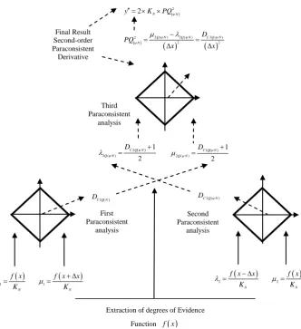
Figure 2shows the sequential for obtain the second-order Derivative Paraconsistent.

4. Application Examples Second-Order Paraconsistent Derivative

1) Example 1

As first example consider the procedure of obtaining the Derivative through Paraconsistent Logical Model, where it is desired a final value of the second-order Paraconsistent Derivative of the function: f x

( )

=x2 in x=3.

Resolution: For the resolution, initially is estimated the maximum function value at the point considered 3

x= .

Therefore, being: f x

( )

=x2 → f x

( )

=ymax →

( )

2

3 9

f x = =

The value of the Paraconsistent Newton Normalization Factor is calculated by Equation (11):

max

2 9 2

N N

K = y →K =

With the Equation (26) is obtained the second-order Paraconsistent Derivative:

( )

_{( )}

(

)

( )

(

)

2 2

1

9 2 9 2 9 2 9 2

2

N

f x x f x f x f x x

PQ

x

ψ

 + ∆   − ∆ 

=  −  − − 

∆    

( )2

_{( )}

(

)

( )

)

(

( )

(

)

2 2 2 2

2

1

3 3 3 3

2 9 2 N

PQ f x f f f x

x

ψ = _{× ×} _∆  + ∆ − − − − ∆ 

Choosing an increment value of variable x such that: ∆ =x 0.001 it comes that:

( )2

₍

₎

(

)

( )

)

(

( )

(

)

2 2 2 2

2

1

3 0.001 3 3 3 0.001

2 9 2 0.001 N

PQ_ψ = _ f + − f − f − f − _

 

(8)

Extraction of degrees of Evidence

Function f x

( )

First Paraconsistent

analysis Third Paraconsistent

analysis Final Result

Second-order Paraconsistent Derivative

Second Paraconsistent

analysis

( )

( ) _{( )} _{( )}

2

2 ( ) 2 ( ) 3 ( ) 2

2 2

2 N N

Q N Q N C Q N N

y K PQ

D PQ

x x

ψ

ψ ψ ψ

ψ

µ λ

′′ = × ×

−

= =

∆ ∆

( )

2 2 ( )

1

2

C Q N Q N

D ψ

ψ

λ = + 1( )

2 ( )

1

2

C Q N Q N

D _ψ

ψ

µ = +

( )

1 C Q N

D DC Q2 (ψN)

( ) ( )

2 2

N N

f x x f x

K K

λ = − ∆ µ =

( ) ( )

1 1

N N

f x f x x

K K

[image:8.595.147.480.80.444.2]

λ= µ = + ∆

Figure 2. Flow of sequential calculation procedure for obtaining the second-order Derivative Paraconsistent.

( )2

₍

₎

2

(

) (

)

1

9.006001 9 9 8.994001 2 9 2 0.001

N

PQ_ψ = _ − − − _

× ×

( )2

₍

₎

2

(

) (

)

( )2

1 0.000002

0.006001 0.005999

0.000025455

2 9 2 0.001

N N

PQ_ψ = _ − _→PQ_ψ =

× ×

Resulting: _{( )}2 0.07856742

N PQ

ψ =

The value of the second-order Paraconsistent Derivative of function f x

( )

in actual physical universe is obtained by applying Equation (27):

( )2

2 _N 2 9 2 0.07856742 2

N

y K PQ

ψ

′′ = × × = × × =

Then, for these conditions of ∆ =x 0.001 the value of the second-order Paraconsistent Derivative of function

( )

2

f x =x in x=3 is: y′′ =2.

2) Example 2

As a second example consider, that one wishes to determine:

a) The first-order Paraconsistent Derivative equation of the function f x

( )

=3x2+1.

(9)

c) The value of the second-order Paraconsistent Derivative of function f x

( )

=3x2+1 in the point x=2.

Resolution:

a) Using the Paraconsistent Newton’s quotient exposed in the form of Equation (13) the function

( )

2

3 1

f x = x + in the Paraconsistent Logical Model is:

( )

(

)

( )

2 2

3 1 3 1

1 N

N N

x x x

PQ

x K K

ψ

 _{+ ∆} ₊ ₊ 

=  − 

∆ _ _

where: PQ₍_ψ_N₎ is the Paraconsistent Newton’s quotient.

KN is the Newton Normalization Factor computed by Equation (11): KN = 2ymax

The Favorable Evidence Degree is:

(

)

2

3 1

N

x x

K

µ= + ∆ +

The Unfavorable Evidence Degree is:

( )

2

3 1

N x

K

λ= +

b) The first-order Paraconsistent Derivative of the function f x

( )

=3x2+1, for x=2 with ∆ =x 0.001, is calculated by sequence:

• Obtaining the maximum value of the function at the point x=2 where:

( )

2

( )

2

max 3 1 max 3 2 1 13

y = x + →y = + =

• The Newton Normalization Factor KN is: KN = 2ymax →KN =13 2

• Applying the Paraconsistent Derivative equation obtained in item a, for ∆ =x 0.001, we have:

( )

(

)

( )

(

)

( )

2 2 2 2

3 1 3 1 3 2 0.001 1 3 2 1

1 1

0.001 13 2 13 2

N N

x x x

PQ PQ

x K K

ψ ψ

 _{+ ∆} ₊ ₊   ₊ ₊ ₊ 

=  − → =  − 

∆ _ _ _ _

( N) _0.0011

[

0.707759658 0.707106781

]

( N) _0.0011

[

0.000652876

]

PQ_ψ = − →PQ_ψ =

( N) 0.652876812

PQ_ψ =

The value of the first-order Paraconsistent Derivative in the physical world is obtained by Equation (12):

( ) 13 2 0.652876812 12.00299415

N N

y′=K ×PQ_ψ → =y′ × =

c) Using the procedures in Paraconsistent Logical Model, the second-order Paraconsistent Derivative function

( )

2

3 1

f x = x + is obtained by Equation (26), where:

( )

_{( )}

(

)

( )

(

)

2

2 2 2 2

2

3 1 3 1 3 1 3 1

1

2 N

N N N N

x x x x x x

PQ

K K K K

x ψ

 _{+ ∆} ₊ ₊   ₊ _{− ∆} ₊ 

   

= − − −

   

 

∆ __ _{ } __

The second-order Paraconsistent Derivative of the function f x

( )

=3x2+1 at the point x = 2 with ∆ =x 0.001 is computed by:

• Obtaining the maximum value of the function at the point x = 2 where:

( )

2

( )

2

max 3 1 max 3 2 1 13

y = x + →y = + =

• The Newton Normalization Factor KN is: KN = 2ymax →KN =13 2

• Applying the Paraconsistent Derivative equation obtained in item a, for ∆ =x 0.001, we have:

( )

₍

₎

(

)

( )

(

)

2

2 2 2 2

2

3 2 0, 001 1 3 2 1 3 2 1 3 2 0, 001 1 1

13 2 13 2 13 2 13 2

2 0.001 N

PQ ψ

 ₊ ₊ ₊   ₊ ₋ ₊ 

   

= − − −

   

_ _{ } _

 

( )2

₍

₎

2

1 13.012003 13.000000 13.00000 12.988003

13 2 13 2 13 2 13 2

2 0.001

N

PQ_ψ = __ −  _{ }− − __

   

(10)

( )2

₍

₎

₂

(

) (

)

( )2 1

0.012003 0.011997 0.163178488

2 0.001 13 2

N N

PQ_ψ = _ − _→PQ_ψ =

The value of the second-order Paraconsistent Derivative in the physical world for the function f x

( )

=3x2+1 at x=2 is obtained by Equation (27):

( )2

2 _N 2 13 2 0.163178488 6

N

y K PQ y

ψ

′′= × × → ′′= × × =

Therefore, for these conditions of ∆ =x 0.001 the value of the second-order Paraconsistent Derivative of function f x

( )

=3x2+1 at x=2 is: y′′ =6.

5. Conclusion

A method for Differential Calculus using the foundations of Paraconsistent Logic applied to the Newton’s quo- tient was presented. As it is seen, the Paraconsistent Differential Calculus is structured in a logic that accepts contradictions; it is able to dissolve the uncertainties, aggregating values that would be conventionally discarded. Following the procedures of Paraconsistent Mathematics it was presented some examples where results are obtained with resolutions of first and of second-order Paraconsistent Derivative of some functions. The results in- dicate that Paraconsistent Mathematics responds well to these basic applications and facilitates the computation- al treatment. Thus it was obtained a model of Paraconsistent Differential Calculus where the results show that the application of Paraconsistent Mathematics responds well to an issue related to non-consideration of infinitesimal. To improve the conclusions, other works which use complex functions should be developed, however, for the equations of the samples the results were quite satisfactory. And the greatest importance of these Paracon- sistent Differential Calculus lies in the fact that, all calculations are based on the concepts of Paraconsistent Logic where contradictions are not ignored, but their values added to the final result.

References

[1] Da Costa, N.C.A. (1974) On the Theory of Inconsistent Formal Systems. Notre Dame Journal of Formal Logic, 15, 497-510. http://dx.doi.org/10.1305/ndjfl/1093891487

[2] Arruda, A.I. (1989) Aspects of the Historical Development of Paraconsistent Logic. In: Priest, G., Routley, R. and Norman, J., Eds., Paraconsistent Logic: Essays on the Inconsistent, Philosophia Verlag, 99-130.

[3] Da Silva Filho, J.I., Lambert-Torres, G. and Abe, J.M. (2010) Uncertainty Treatment Using Paraconsistent Logic: In-troducing Paraconsistent Artificial Neural Networks. IOS Press, Amsterdam.

[4] Jas’kowski, S. (1969) Propositional Calculus for Contradictory Deductive Systems. Studia Logica, 24, 143-157.

http://dx.doi.org/10.1007/BF02134311

[5] Da Silva Filho, J.I. (2011) Paraconsistent Annotated Logic in Analysis of Physical Systems: Introducing the Paraquan- tum hψ Factor of Quantization. Journal of Modern Physics, 2, 1397-1409.

http://dx.doi.org/10.4236/jmp.2011.211172

[6] Da Costa, N.C.A. (2000) Paraconsistent Mathematics. In: Batens, D., Mortensen, C., Priest, G. and van Bendegen, J.P., Eds., I. World Congress on Paraconsistency, 1998 Ghent, Belgium. Frontiers in Paraconsistent Logic: Proceedings, King’s College Publications, London, 165-179.

[7] Da Silva Filho, J.I. (2011) Paraconsistent Annotated Logic in Analysis of Physical Systems: Introducing the Paraquan- tum γψ Gamma Factor. Journal of Modern Physics, 2, 1455-1469. http://dx.doi.org/10.4236/jmp.2011.212180

[8] Stroyan, K.D. and Luxemburg, W.A.J. (1976) Introduction to the Theory of Infinitesimals. Academic Press, New York.

[9] Pl Tipler, A. and Llewellyn, R.A. (2007) Modern Physics. 5th Edition, W. H. Freeman and Company, New York.

[10] Diethelm, K. and Ford, N. (2004) Multi-Order Fractional Differential Equations and Their Numerical Solution. Applied Mathematics and Computation, 154, 621-640. http://dx.doi.org/10.1016/S0096-3003(03)00739-2

[11] Bell, J.L. (1998) A Primer of Infinitesimal Analysis. Cambridge University Press, Cambridge.

[12] Baron, M.E. (1969) The Origins of the Infinitesimal Calculus. Pergamon Press, Hungary.