A Genetic Algorithm Approach using Improved Fitness
Function for Classification Rule Mining
Salma-Tuz-Jakirin
MS Student Department of Computer Science and Engineering
University of Dhaka, Bangladesh
Abu Ahmed Ferdaus
Assistant Professor Department of Computer Science and Engineering
University of Dhaka, Bangladesh
Mehnaj Afrin Khan
MS Student Department of Computer Science and Engineering
University of Dhaka, Bangladesh
ABSTRACT
Classification rule mining from huge amount of data is a challenging issue in data mining. Classification rules describe the relationship between predicting attributes and class label attribute and thus assign class label to unseen predicting attribute values. In this paper, a Genetic algorithm approach with modified fitness function for discovering classification rules has been presented. A flexible encoding scheme for representing a rule, genetic operators like crossover, mutation and also the stated fitness function with confidence, coverage, simplicity and interestingness properties have been exploited for discovering accurate, comprehensible and interesting rules. The results of proposed Genetic algorithm have been compared with existing J48, Jrip, Naive Bayesian algorithms. Experimental results endorse that the proposed algorithm produces relatively less number of classification rules with satisfactory accuracy rates.
General Terms
Classification, Data mining, Classification rules
Keywords
Genetic Algorithm, Crossover, Mutation, Fitness function
1.
INTRODUCTION
The data and information of our real life activities play a significant role in the field of data mining. In this era of information technology, huge amount of data are storedin the databases from different ends and the rapidly growing massive data with enormous size makes the job harder for an organization or researchers to discover knowledge from the large databases. Data mining is a core process for analyzing data and extracting valuable hidden knowledge from huge amount of data. Rule mining is one of the key methods to explore valuable knowledge from the large databases. Classification is one of the major domains of data mining which discovers rules for classification as well as assigns instances to a specificclass. The purpose of classification is to correctly predict the class label for each case in the data. Different types of data mining techniques like Decision tree, Neural network, Naïve Bayesian, Genetic algorithms and Support Vector Machine etc. exist for classification. Genetic algorithms [1, 2, 3, 4] is based on biological mechanism and takes attention of attribute interactions and has the capability of avoiding the convergence to local optimal solutions.
2.
RELATED WORK
A set of approaches have been studied for understanding the discovery of classification rules in data mining field. Some of those are described sequentially in this section.
2.1
C4.5
Quinlan proposed C4.5 algorithm [5, 6] for generating C4.5 decision tree. C4.5 can handle discrete and continuous attribute values and also missing values. It uses greedy technique to generate decision tree which also provides the opportunity for pruning the tree further. The C4.5 can choose irrelevant attribute which may affect badly the construction of a decision tree. J48 is a Java implementation of C4.5 algorithm.
2.2
RIPPER
RIPPER (Repeated Incremental Pruning to Produce Error Reduction) [7] is based on the incremental reduced error-pruning. Ripper algorithm learns single rule using information gain. The algorithm is easy to understand and usually better than decision tree learning. The algorithm scales poorly with increased training set size and creates problems with noisy data.
2.3
Naive Bayesian
In Naive Bayesian algorithm [5], the class membership probability is predicted using the concept of conditional probabilities. Bayes theorem with strong independence assumption is applied to classifier. Advantages include high accuracy and speed, highly scalable building model, classification of both binary and multiclass data and also parallelism. Again loss of accuracy may incur because of assumption of independence of feature, since dependencies can exist among attributes in reality.
2.4
Neural Network
The classification in Neural network [5] can be done by Backpropagation. The network is developed based on operation of human neural system. The advantages include robustness, high accuracy rate and the output which can be real, discrete or combination of real and discrete attributes. The Neural network requires parameters for creating network and it is not easy to define no. of layers, nodes, weights etc. The learning function is also difficult to understand.
3.
PROPOSED GENETIC ALGORITHM
populations using an iteration approach. For the generation of new population, a fitness function is used to evaluate the quality. Better individuals are discovered by an iterative procedure where each iteration utilizes a selection method of individuals using genetic operators like crossover and mutation. The main target of using the GA is to find out high level classification rules. GA performs global search which leads to handle better attribute interactions than the traditional search methods.
Before applying Genetic algorithm, some preprocessing steps should be done. After the preprocessing steps, Genetic algorithm has to be implemented. The process of the Genetic algorithm is below:
1. Create population based on database and find out fitness values of each member of the population.
2. Apply the genetic operators on the population and create new population.
3. After comparing the two generations of populations, best population is discovered.
4. After running several generations, final population can be realized. This population is the classification rules.
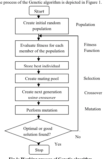
The process of the Genetic algorithm is depicted in Figure 1.
No
[image:2.595.63.277.326.651.2]
Fig 1: Working process of Genetic algorithm
3.1
Preprocessing
Preprocessing includes discritization of continuous attribute values, selection of perfect or proper attribute and separation of dataset to training and testing tuples.
3.1.1
Discretization of Continuous Attribute
Entropy based discretization method [5] is used for discretization which is based on supervised learning and that uses top-down splitting approach. It also uses class distribution information for entropy calculation. For
discretization, a split point is chosen. Split point is a value of a continuous attribute. Using split point, the dataset is divided into two parts.
The equation for calculating expected information requirement is
Here, D1 contains the records satisfying the condition A
split point. D2 also contains the records satisfying the
condition A > split point. The number of total records is contained in |D|. Based on class distribution of the records, entropy function is calculated.
The equation for calculating entropy function for m classes
of is given bellow:
Here, is the probability of class in .
3.1.2
Attribute Selection
For feature or attribute selection, two types of technique are used like filter approach and wrapper approach [8]. In this research, wrapper approach is implemented which depends on data mining algorithm for attribute selection.
3.1.2.1
Calculation of Entropy
Initial population is generated by calculating entropy for each attribute. Using this value, informative attributes can be found which can produce best classification rules [4]. The equation for calculating entropy of an attribute is:
Where, is the entropy value of attribute and v is the number of values the Attribute can take. The number of classes is represented by n. For classifying a record, the expected information is given by second term. The weight of
partition is given by .
3.1.2.2
Calculation of Probability of Initialization
After calculating entropy, probability of initialization is calculated through linear transformation. The entropy of attribute which has minimum value initializes with a probability 1 and gets chance to become a part for every classification rule. The attribute which has maximum value initializes with a probability 0. The others attributes are assigned probability of initialization between 0 and 1. The equation for calculating probability of initialization for a attribute is[4]:
where, is the entropy
value of attribute.
3.2
The Procedure of the Genetic Algorithm
3.2.1
Representation of Population
The rules representation step defines how the classification rules are represented for better understanding. The encoding step represents the rules for working with Genetic algorithm approach.
3.2.1.1
Rules Representation
Classification rules are represented by an individual. Several structures of classification rules are suggested by researchers Stop
Start
Create initial random population
Evaluate fitness for each member of the population
Store best individual
Create mating pool
Create next generation using crossover
Perform mutation
Optimal or good solution found?
Selection
Crossover
Mutation
No Yes
Population
[9]. Each Classification rules is divided into two parts: the antecedent part contains predicting attribute values and consequent part contains goal attribute value. The form of rules is:
IF <antecedent> ELSE <consequent>
3.2.1.2
Encoding
Each rule represents an individual of population in Genetic algorithm approach. For encoding a rule into an individual, a binary bit representation is used. Each bit in the individual represents each value of an attribute. If the number of values of an attribute is n, then n number is needed to represent the attribute in binary bit notation. In encoding a rule to an individual, we use Michigan approach [1]. In this approach, a single rule is encoded in each individual. The encoding scheme can be explained by a self devised dataset mentioned in Table 1.
Table 1: Information of Professional Dataset Name of Attribute Values of Attribute
Qualification Educated, Uneducated, Highly educated
Location City, Rural
Family Background High, Low, Medium
Age 20-30, 31-40, 41-50
Class Job, Business, Immigrant
Table 2: Professional Dataset
Qualificat-ion
Loc-ation
Family Background
Age Class
Educated City High 20-30 Immigrant
Uneducated City Low 20-30 Job
Educated Rural Medium 41-50 Business
Highly Educated
City High 31-40 Immigrant
Highly Educated
City Medium 41-50 Job
Uneducated Rural Low 31-40 Job
Educated City Low 41-50 Job
Highly Educated
Rural Medium 20-30 Business
Educated City Medium 31- 40 Job
Uneducated City Medium 41-50 Immigrant
From Table 2, a rule likes this: IF (Qualification = 'Uneducated' and Family Background = 'Low') THEN Class = 'Job' can be found. The bit representation of this rule is as follows:
Table 3: Bit Representation of a Rule
Individual(Bit Representation) Class
01000010000 1
3.2.2
Applying Genetic Operators
To create a new generation using proposed genetic algorithm, crossover and mutation have been used. Before applying crossover and mutation, the individuals are chosen by selection procedure.
3.2.2.1
Selection Procedure
Selection procedure is the stage in which the basis is created for selection of individual. In Genetic algorithm, individuals are chosen for crossover or mutation in such a way that better individual can represent the next generation. In this research, roulette wheel [10] selection method has chosen for selection procedure which is based on fitness value and used for selection of better individual or solution for recombination. It discovers potentially useful solution.
3.2.2.2
Crossover
Crossover is a process to produce new offspring from more than one parent. In this process, genetic material from one parent is combined with genetic material from another parent to discover better offspring. One-point crossover [11] is used in the research work. For example, Professional dataset is taken for representing the crossover process. Here, rule is represented by individual bit representation.
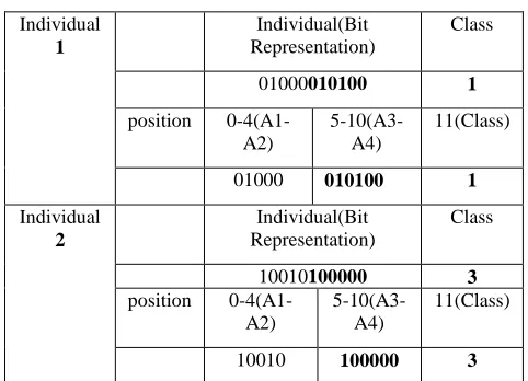
[image:3.595.308.549.427.601.2]For example, in Table 4, crossover is occurred in the position of 5. Attribute A3 starts in the position of 5. In Table 4, the corresponding rule for individual 1 is IF(Qualification = 'Uneducated' and Family Background = 'Low' and Age = ’20-30’) THEN Class = 'Job' and for individual 2 is IF(Qualification = 'Educated' and Location = ‘City’ and Family Background = ‘High') THEN Class = 'Immigrant' .
Table 4: Before Crossover
Individual
1
Individual(Bit Representation)
Class
01000010100 1
position 0-4(A1-A2)
5-10(A3-A4)
11(Class)
01000 010100 1
Individual
2
Individual(Bit Representation)
Class
10010100000 3
position 0-4(A1-A2)
5-10(A3-A4)
11(Class)
10010 100000 3
After crossover, in Table 5, the corresponding rule for individual 1 is IF(Qualification = 'Uneducated' and Family Background = 'High') THEN Class = 'Immigrant' and for individual 2 is IF(Qualification = 'Educated' and Location = ‘City’ and Family Background = 'Low' and Age = ’20-30’) THEN Class = 'Job' .
Table 5: After Crossover
Individual
1
Individual(Bit Representation)
Class
01000100000 3
A2) A4)
01000 100000 3
Individual
2
Individual(Bit Representation)
Class
10010010100 1
position 0-4(A1-A2)
5-10(A3-A4)
11(Class)
10010 010100 1
3.2.2.3
Mutation
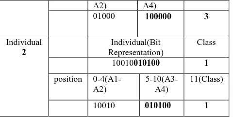
Mutation is the process for maintaining the genetic diversity. By inserting or removing conditional clauses into a rule antecedent, this operator may specialize or generalize a rule. In this process, one value of the individual is altered. After mutation, the individual is changed to new individual. For example, in Table 6, in the bit position 8 where one value of attribute 4(A4) is 1. After mutation, this bit is changed to 0.
[image:4.595.49.289.72.193.2]In table 6, before mutation the corresponding rule for individual is IF(Qualification = 'Uneducated' and Family Background = 'Low' and Age = ’20-30’) THEN Class = ‘Job' and after mutation the corresponding rule for individual is IF(Qualification = 'Uneducated' and Family Background = 'Low' ) THEN Class = 'Job' .
Table 6: Mutation
Before
Individual(Bit Representation)
Class
01000010100 1
position 0-4(A1-A2) 5-10(A3-A4)
11(Class)
01000 010100 1
After
Individual(Bit Representation)
Class
01000010000 1
position 0-4(A1-A2) 5-10(A3-A4)
11(Class)
01000 010000 1
3.2.3
Fitness Evaluation Function
For evaluating the quality of a rule, fitness functions are used in Genetic algorithm. For discovering accurate, comprehensible and interesting rules, various measures are related. In this research, confidence, coverage, simplicity and measurement of interesting factor are chosen. A rule's representation is
IF X THEN where X is antecedent part and is consequent part.
3.2.3.1
Precision
The Precision (or confidence) of a rule is the ratio of the number of records in X which are correctly classified as goal class of is defined as precision.
3.2.3.2
Coverage
The Coverage of a rule is the ratio of the number of records in X which are correctly classified as goal class of and the number of records satisfying is defined as coverage.
3.2.3.3
Complexity
The number of attributes on the antecedent part defines the complexity of a rule. The complexity of the rule can be defined as:
Complexity = number of attributes in antecedent part of rule
3.2.3.4
Interestingness
The measurement of rule interesting is calculated as follows:
From this equation, we get, is the number of records that assure that both antecedent part and consequent part(class label) will be satisfied.
3.2.3.5
Proposed Fitness Function
The modified fitness function of a rule that we incorporated in the Genetic algorithm is as follows:
4.
PERFORMANCE ANALYSIS
4.1
Performance Study
In this section, the performance of the proposed Genetic algorithm is represented. The objective of this research is to discover accurate and interesting classification rules. The results of proposed Genetic algorithm were compared with the results of J48 [5], JRip [7] and Naive Bayesian [5] algorithms. For this purpose, Weka [12] implementation of J48, JRip and Naïve Bayesian algorithms were exercised. All the experiments were conducted on a 2.93GHz Intel(R) Core(TM)2 Duo CPU with 4GB RAM on Microsoft Windows 7 environment.
4.2
Experimental Study
The experiment was designed in three steps:The first step was preprocessing step. In this step, the tuples with missing attributes were removed and continuous attributes were discretized. The entropy of each attribute and probability of initialization of each attribute for relevant attribute selection were also calculated in this step.
In the second step, the proposed Genetic algorithm was applied in the datasets.
The last step was post-processing step. In this step, the coverage for each rule was calculated and the final rules were discovered according to this measure. All results were taken as average of 10 runs of Genetic algorithm. The best scores were taken for final results. That is, these best scores provided the best rules with the help of Genetic algorithm.
4.3
Characteristics of rules
label creates the consequent part. The rules were represented by IF...THEN statement. The IF statement included the conjunction among different predicting attributes and disjunction among same predicting attribute values. That is, the different predicting attributes were joined in the IF statement using 'and' operator and the same predicting attribute values were joined using 'or' operator. In the THEN statement, only one value of goal attribute was present that defined the class label for classifying instances.
4.4
Datasets
For the experiment, six classification datasets were used. All experimental datasets were obtained from UCI Machine Learning Repository [13], a collection of real-world datasets for data mining. The properties of these datasets are shown in Table 7.
Table 7: Properties of Experimental Datasets
Dataset No. of Instances
No. of Attributes
No. of Classes
Nursery 12960 8 5
Car 1728 6 4
Breast Cancer 286 9 2
Qualitative Bankruptcy
250 7 2
Iris 150 4 3
Lenses 24 4 3
For discovering classification rules, the list of parameters for Genetic algorithm is given in Table 8.
Table 8: The List of Parameters for Experiment
Dataset Crossover probability
Mutation Probability
No. of Gener-ations
Population Size
Nursery 0.7 0.1 300 60
Car 0.6 0.1 250 50
Breast Cancer
0.8 0.1 100 40
Qualitative Bankruptcy
0.8 0.1 200 70
Iris 0.5 0.1 200 60
Lenses 0.65 0.1 150 55
4.5
Result Analysis
4.5.1
Accuracy Rates
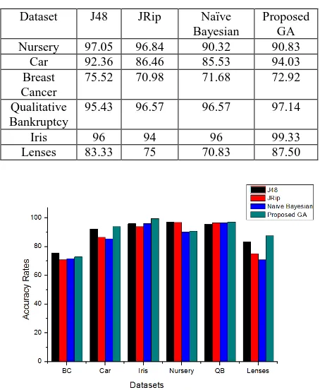
To measure the classifier’s performance, the accuracy rates are measured. When the classifier correctly predicts the class of each instance or record then it is correctly classified; otherwise it creates an error. The accuracy rates is made over a whole set of instances with the number of correctly classified instances. From Figure 2, the accuracy rates of the JRip, Naive Bayesian and J48 and the proposed Genetic algorithms can be observed. The proposed algorithm offered the best result for iris dataset. For car, qualitative bankruptcy and lenses dataset, the proposed algorithm depicted the better results than other algorithms. The accuracy rates for car, qualitative bankruptcy, lenses and iris dataset were 94.03%, 97.14%, 87.50% and 99.33% respectively which were better than the accuracy rates of JRip, Naive Bayesian and J48 algorithms. The observation also notified that the proposed Genetic algorithm did not achieve the best results for all datasets. For nursery and breast cancer datasets, the algorithm
[image:5.595.315.542.109.385.2]provided the less accuracy rates than JRip and J48. Table 9 lists the accuracy rates on experimental datasets.
Table 9: Accuracy Rates in Percentage (%)
Dataset J48 JRip Naïve Bayesian
Proposed GA Nursery 97.05 96.84 90.32 90.83
Car 92.36 86.46 85.53 94.03
Breast Cancer
75.52 70.98 71.68 72.92
Qualitative Bankruptcy
95.43 96.57 96.57 97.14
Iris 96 94 96 99.33
Lenses 83.33 75 70.83 87.50
Fig 2: Accuracy Rates on Experimental Datasets
4.5.2
Number of Rules
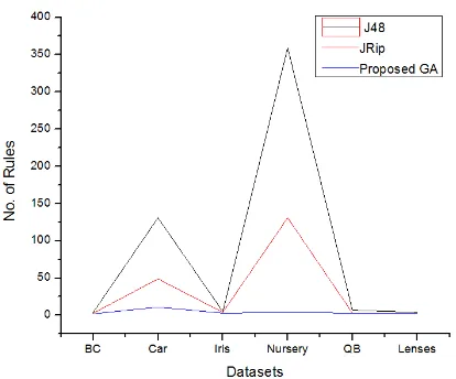
[image:5.595.316.549.531.629.2]From Table 10 and Figure 3, the number of classification rules could be observed. It also noticed that, the proposed Genetic algorithm derived the minimum number of classification rules than other algorithms. This indicated the proposed Genetic algorithm can classify many instances using a small number of rules whereas the others required more rules. Finally it can be conclude that the proposed Genetic algorithm generated less number of classification rules without sacrificing significant accuracy.
Table 10: Number of Rules
Dataset J48 Jrip Proposed GA
Nursery 359 131 4
Car 131 49 11
Breast Cancer 4 3 2
Qualitative Bankruptcy
7 3 3
Iris 5 4 3
Fig 3: No. of Rules on Experimental Datasets
4.5.3
Discovered Rules
The discovered classification rules for each experimental datasets are given below:
4.5.3.1
Nursery Dataset
Table 11: Rules of Nursery Dataset Discovered Rules
IF health = not recom THEN class = not recom
IF health = recommended or priority THEN class= spec prior IF parents = pretentious and health = recommended or priority THEN class = priority
IF parents = usual and health = recommended or priority THEN class = priority
4.5.3.2
Lenses Dataset
Table 12: Rules of Lenses Dataset Discovered Rules
IF TEAR PRODUCTION RATE = 1 THEN class = 3
IF ASTIGMATIC = 1 and TEAR PRODUCTION RATE = 2 THEN class = 2
IF ASTIGMATIC = 2 and TEAR PRODUCTION RATE = 2 THEN class = 1
4.5.3.3
Car Dataset
Table 13: Rules of Car Dataset
[image:6.595.60.267.77.249.2]4.5.3.4
Qualitative Bankruptcy Dataset
Table 14: Rules of Qualitative Bankruptcy Dataset Discovered Rules
IF competitiveness = A or P THEN class = NB IF competitiveness = N THEN class = B
IF competitiveness = A and creditibility = N and financial flexibility = N THEN class = B
4.5.3.5
Iris Dataset
Table 15: Rules of Iris Dataset Discovered Rules
IF petal length = > 1.9 and petal width = > 0.6 THEN class = Iris-virginica
IF sepal width = 3.3 and petal length = > 1.9 and petal width = > 0.6 THEN class = Iris-versicolor
IF petal length = 1.9 and petal width = 0.6 THEN class = Iris-setosa
[image:6.595.46.290.306.736.2]4.5.3.6
Breast Cancer Dataset
Table 16: Rules of Breast Cancer Dataset Discovered Rules
IF DEG MALIG = 1 or 2 THEN class = no-recurrence-events IF DEG MALIG = 3 THEN class = recurrence-events
5.
CONCLUSION
The proposed Genetic algorithm can be used to find classification rules from classification databases. To achieve this purpose, the proposed algorithm used different measures like precision, coverage, complexity and interestingness to evaluate the quality of a rule based on fitness function. After evaluation, fittest rules were discovered for the experimental datasets. From this research, impressive accuracy rates with less number of classification rules were also found. In future, the goal is to try to explore datasets having large number of attributes and optimize several parameters like crossover rate, mutation rate etc. and thus investigate the scope to improve the quality of the proposed algorithm. Again, in this research, single objective genetic algorithm was used. The multi objective genetic algorithm can be designed for discovering classification rule as future extension of this research.
6.
REFERENCES
[1] A. Freitas, “A survey of evolutionary algorithms for data mining and knowledge discovery”, In: A. Ghosh, and S. Tsutsui (Eds.) Advances in Evolutionary Computation. Springer-Verlag, 2002.
[2] B. M. A. Al-Maqaleh, “Genetic algorithm approach to automated discovery of comprehensible production rules," Advanced Computing and Communication Technologies, International Conference on, vol. 0, pp. 69-71, 2012.
[3] M. A. jabbar, B. Deekshatulu, and P. Chandra, “Classification of heart disease using k- nearest neighbor and genetic algorithm,” Procedia Technology, vol. 10, pp. 85-94, 2013, first International Conference on Computational Intelligence: Modeling Techniques and Applications (CIMTA) 2013.
Discovered Rules
IF safety = high THEN class= vgood
IF persons = 2 and safety = high THEN class = unacc IF safety = low THEN class = unacc
IF persons = 2 and safety = med THEN class = unacc IF lug boot = small and safety = med THEN class = unacc IF safety = med THEN class = acc
IF persons = 4 and safety = high THEN class = acc IF persons = more and safety = high THEN class = acc IF maint = low and safety = med THEN class = good IF lug-boot = big and persons = 4 and safety = med THEN class = good
[4] Kapila, Saroj, D. Kumar, and Kanika, “A genetic algorithm with entropy based initial bias for automated rule mining," in International Conference on Computer and Communication Technology, 2010.
[5] J. Han, M. Kamber, and J. Pei, Data Mining: Concepts and Techniques, 3rd ed. San Francisco, CA, USA: Morgan Kaufmann Publishers Inc., 2011.
[6] R. J. Quinlan, “Learning with continuous classes," in 5th Australian Joint Conference on Artificial Intelligence. Singapore: World Scientific, 1992, pp.343-348.
[7] W. W. Cohen, “Fast effective rule induction," in Proceedings of the 12th International Conference on Machine Learning, 1995.
[8] J. Huang, Y. Cai, and X. Xu, “A wrapper for feature selection based on mutual information." IEEE Computer Society, 2006, pp. 618-621.
[9] Yogita, Saroj, D. Kumar, and Vipin, “Rules + Exceptions: Automated Discovery of Comprehensible Decision Rules," in IEEE International Advance Computing Conference, 2009.
[10]Web link: Roulette wheel selection http://www.edc.ncl.ac.uk/highlight/rhjanuary2007g02.ph p (last accessed on April 15, 2014).
[11]Web link: Crossover (genetic algorithm) http://en.wikipedia.org/wiki/Crossover_(genetic_algorith m) (last accessed on April 16, 2014).
[12]Web link: Weka 3: Data mining software in java http://www.cs.waikato.ac.nz/ml/weka/ (last accessed on April 25, 2014).