New Fangled Mandelbrot and Julia Sets for Logarithmic Function

(1)

New-Fangled Mandelbrot and Julia Sets for Logarithmic

Function

Suraj Singh Panwar

M.Tech. - CSE, Scholar Faculty of Technology,

Computer Science and Engineering Department, Uttarakhand Technical University, Dehradun

Pawan Kumar Mishra

Assistant Professor, M.Tech. CSE

Faculty of Technology,

Computer Science and Engineering Department, Uttarkhand Technical University, Dehradun

ABSTRACT

In this paper we explore the dynamics of complex logarithmic function for integer and non-integer values. We have used Ishikawa iteration method for generating fractals and analyzed them.

Keywords

Fractals, Mandelbrot set, Julia set, Mann Iteration, Ishikawa Iteration, Computer Graphics, Fixed point and Graph.

1. INTRODUCTION

Fractal Theory is an exciting branch of applicable Mathematics and Computer Science. It is based on the concept of self-similar forms. Benoit Mandelbrot (1924-2010), scientist and mathematician who also worked at IBM, is known as the father of fractal geometry. Mandelbrot coined the word fractal in the late 1970s. Mandelbrot published to explain geometric fractals as "a rough or fragmented geometric shape that can be divided into parts, every one of which is a reduced-size duplicate of the whole".[1] There are many sort of fractals found in nature. Fractals are all around us in the form of many usual objects such as mountains, coastlines, trees ferns and clouds [2,3,4]. They all are fractals in nature and can be represented on a computer by a recursive algorithm of computer graphics. Before the innovation of computers, Fractals have appeared as an important question. Fractal is defined as a set, which is self– similar under magnification.[5]

The Julia sets and the Mandelbrot sets are two most important objects under various researches in the field of fractal theory [6]. The Julia set was given by French mathematician Gaston Julia (1893-1978) in 1918, whereas the Mandelbrot set was given by Benoit B. Mandelbrot (1924-2010) in 1979.

2. PRELIMINARIES

2.1 Mann’s Iteration: One Step Iteration

Mann’s iteration technique is a one-step iteration technique given by William Robert Mann (1920-2006), a mathematician from Chapel Hill, North Carolina. The iteration technique involves one step for iteration, and is given as [7,8]:

xn+1 = (1-s)xn + s.f(xn),

where n≥0 and 0 < s < 1

2.2 Ishikawa Iteration : Two Step Iteration

Ishikawa iteration [9,10] technique is a two-step iteration method known after Ishikawa. Let X be a subset of complex number and f : X→X for all x0 ϵ X , we have the sequence

numbers for {xn} and {yn} in X according to following way.

[11,12] :

'

(

) (1

' )

n n n n n

y



S

f x

 

S

x

1

(

) (1

)

n n n n n

x

_



S f y

 

S x

Where, 0 ≤S’n ≤ 1, 0 ≤ Sn≤ 1 and S’n & Sn are both convergent

to non-zero number.

3. GENERATION OF RELATIVE

SUPERIOR MANDELBROT SETS

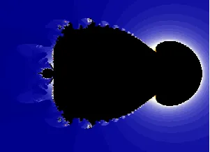
We present here some Relative Superior Mandelbrot sets for the function Z log(Zn+C), n>=2.0, for integer and some non-integer values. Process of generating fractal images is similar to self-squared function [13,14,15]. The parameter s and s’ also changes the structure and beauty of fractals.

3.1 Relative Superior Mandelbrot sets for

[image:1.595.329.512.393.524.2]

Quadratic function:

Figure. 1 Relative Superior Mandelbrot set for s=s’=1,n=2

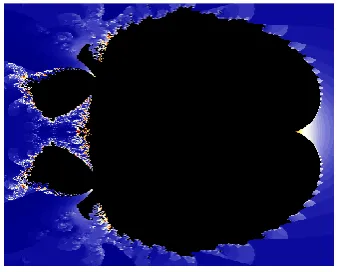
[image:1.595.352.503.555.664.2]

(2)

[image:2.595.83.257.70.215.2] [image:2.595.340.511.107.247.2]

Figure 3 Relative Superior Mandelbrot set for s=s’=1,n=2.4

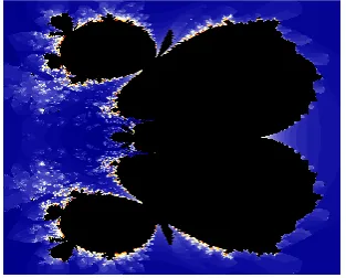
[image:2.595.92.247.244.394.2]

Figure 4 Relative Superior Mandelbrot set for s=s’=1,n=2.8

Figure 5 Relative Superior Mandelbrot set for s=s’=0.5, n=2.4

Figure 6 Relative Superior Mandelbrot set for s=s’=0.5,n=2.8

3.2 Relative Superior Mandelbrot set for

Cubic function.

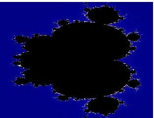
[image:2.595.342.516.274.396.2]

Figure 7 Relative Superior Mandelbrot set for s=s’=1, n=3.

[image:2.595.344.510.422.553.2]

Figure 8 Relative Superior Mandelbrot set for s=s’=0.5,n=3

Figure 9 Relative Superior Mandelbrot set for s=s’=1, n=3.4

[image:2.595.343.509.582.732.2] [image:2.595.85.255.588.724.2]

(3)

[image:3.595.92.247.70.213.2]

3.3 Relative Superior Mandelbrot set for

[image:3.595.352.499.71.211.2]

Bi-Quadratic function.

Figure 13 Relative Superior Mandelbrot set for s=s’=1,n=4

Figure 14 Relative Superior Mandelbrot set for s=s’=0.5,n=4

[image:3.595.349.506.417.557.2]

Figure 15 Relative Superior Mandelbrot set for s=s’=1,n=4.4

[image:3.595.102.260.442.572.2]

[image:3.595.341.511.588.724.2]

Figure 17 Relative Superior Mandelbrot set for s=s’=0.5,n=4.4

[image:3.595.92.249.603.729.2]

(4)

[image:4.595.347.507.72.227.2]

3.4 Generalization of Relative Superior

Mandelbrot sets:-

[image:4.595.92.250.108.237.2]

[image:4.595.348.505.258.378.2]

[image:4.595.92.249.267.387.2]

[image:4.595.336.514.423.556.2]

[image:4.595.333.519.587.731.2] [image:4.595.98.244.587.736.2]

(5)

4. GENERATION OF RELATIVE

SUPERIOR JULIA SETS

We present here some Relative Superior Julia sets for the function Z log(Zn+C), n>=2.0, for integer and some non-integer values. The parameter s and s’ also changes the structure and beauty of fractals. Following are some of the Julia sets for quadratic, cubic and bi-quadratic functions.

4.1 Relative Superior Julia sets for

[image:5.595.332.519.72.194.2]

Quadratic function.

Figure 27 RSJS for s=s’=0.5, n=2, c=0.21527778+ 0.00694444i

Figure 28 RSJS for s=s’=.5,n=2.5 c=0.2152777778+ 0.0069444444i

4.2 Relative Superior Julia sets for Cubic

function.

Figure 29 RSJS for s=s’=1,n=3 c=0.5234- 0.6319i

Figure 30 RSJS for s=s’=1, n=3.5 c=0.5234-0.6319i

4.3 Relative Superior Julia sets for

[image:5.595.61.264.162.331.2]

Bi-Quadratic function.

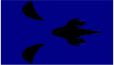
Figure 31 RSJS for s=s’=1,n=4 c=0.423611+0.01388i

Figure 32 RSJS for s=s’=1,n=4.5 c=0.423611+0.01388i

[image:5.595.349.541.257.395.2]

5. FIXED POINTS AND GRAPHS

5.1 Fixed points of quadratic polynomials

Table 1: Orbit of F(z) at s=s’=0.5, n=2 for z0=0.21527778+

0.00694444i

No. of iteration |F(z)| No. of iteration |F(z)|

25 2.5344 35 2.5400

26 2.5355 36 2.5401

27 2.5364 37 2.5400

[image:5.595.71.269.369.482.2] [image:5.595.77.264.560.678.2]

(6)

29 2.5381 39 2.5399

30 2.5390 40 2.5398

31 2.5392 41 2.5398

32 2.5398 42 2.5397

33 2.5398 43 2.5397

34 2.5401 44 2.5397

We skipped 24 Iterations and after 42 iterations value converges to a fixed point.

Figure 33 Orbit of F(z) at s=s’=0.5, n=2 for z0=0.21527778+

0.00694444i

Table 2 : Orbit of F(z) at s=s’=0.5, n=2.5 for z0=0.21527778+0.00694444i

103 2.8276 114 2.8280

104 2.8277 115 2.8280

105 2.8277 116 2.8280

106 2.8278 117 2.8280

107 2.8278 118 2.8280

108 2.8279 119 2.8280

109 2.8279 120 2.8280

110 2.8280 121 2.8280

111 2.8280 122 2.8279

112 2.8280 123 2.8279

113 2.8280 124 2.8279

[image:6.595.318.533.69.243.2]

We skipped 102 Iterations and after 122 iterations value converges to a fixed point.

Figure 34 Orbit of F(z) at s=s’=0.5, n=2.5 for z0=0.21527778+0.00694444i

5.2 Fixed points of Cubic polynomials

Table 3: Orbit of F(z) at s=s’=1, n=3 for z0=0.5234-0.6319i

13 4.5084 23 4.4869

14 4.5014 24 4.4867

15 4.4967 25 4.4866

16 4.4934 26 4.4866

17 4.4912 27 4.4865

18 4.4896 28 4.4865

19 4.4886 29 4.4865

20 4.4879 30 4.4864

21 4.4874 31 4.4864

22 4.4871 32 4.4864

We have skipped 12 Iterations and after 30 iterations value converges to a fixed point.

Figure 35: Orbit of F(z) at s=s’=1, n=3 for z0

(7)

Table 4: Orbit of F(z) at s=s’=1, n=3.5 for z0

=0.5234-0.6319i

1 0.8205 12 6.5976

2 3.2012 13 6.6015

3 4.366 14 6.6035

4 5.3174 15 6.6046

5 5.9097 16 6.6051

6 6.2369 17 6.6054

7 6.411 18 6.6056

8 6.5028 19 6.6057

9 6.5512 20 6.6057

10 6.5769 21 6.6058

11 6.5904 22 6.6058

[image:7.595.46.293.86.469.2]

After21 iterations the value converges to a fixed point.

Figure 36: Orbit of F(z) at s=s’=1, n=3.5 for z0

=0.5234-0.6319i

5.3 Fixed points of Bi-quadratic polynomials

Table 5: Orbit of F(z) at s=s’=1, n=4 for

z0=0.423611+0.01388i

1 0.4238 12 8.6053

2 3.1621 13 8.6092

3 4.6181 14 8.6111

4 6.1321 15 8.6119

5 7.2585 16 8.6123

6 7.9297 17 8.6125

7 8.2825 18 8.6126

8 8.4563 19 8.6126

9 8.5394 20 8.6126

10 8.5785 21 8.6127

11 8.5967 22 8.6127

After 21 iterations the value converges to a fixed point.

[image:7.595.314.535.287.660.2]

Figure37:Orbit of F(z) at s=s’=1, n=4 for z0=0.423611+0.01388i

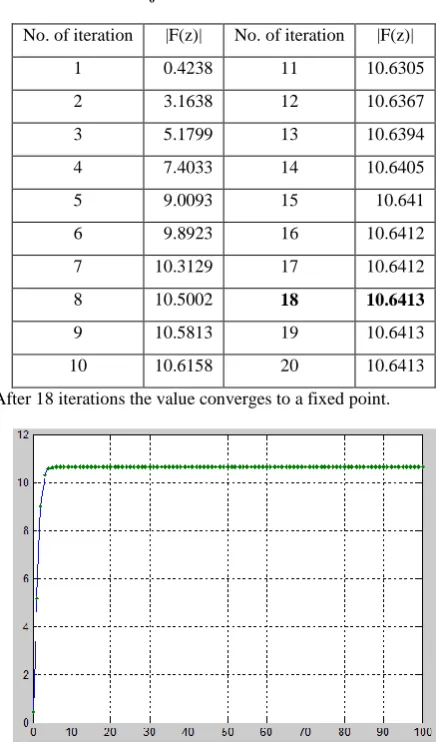
Table 6: Orbit of F(z) at s=s’=1, n=4.5 for z0=0.423611+0.01388i

1 0.4238 11 10.6305

2 3.1638 12 10.6367

3 5.1799 13 10.6394

4 7.4033 14 10.6405

5 9.0093 15 10.641

6 9.8923 16 10.6412

7 10.3129 17 10.6412

8 10.5002 18 10.6413

9 10.5813 19 10.6413

10 10.6158 20 10.6413

After 18 iterations the value converges to a fixed point.

Figure 38: Orbit of F(z) at s=s’=1, n=4.5 for z0=0.423611 +

0.01388i

6. CONCLUSION

(8)

is (n-1). For higher values of n, the central body is bifurcated into (n-1) lobes from left side.

For non integer values, the new lobe is created step by step as it passes to upper integer (ceil) value. From observation and figure shown above, i.e. for n=2, number of lobe is 1 (n-1), as the value of n is increased to 2.4, 2.8, the new lobe is created slowly, and for n=3 there are 2 lobes created from the left portion. So the bifurcation process is seen clearly during non-integer values. The fractals generated are symmetrical along the x-axis. We obtained fixed point for quadratic function after 42 iterations, for cubic function after 30 and for bi-quadratic function after 21 iterations. Similarly we obtained fixed point for n=2.5 after 122 iterations, for n=3.5 after 21 iterations and for n=4.5 after 18 iterations.

7. REFERENCES

[1] Mandelbrot, Benoit B., “The fractal geometry of nature.” Macmillan. ISBN 978-0-7167-1186-5, 1983.

[2] Barnsley, Michale F., Devaney, Robert L., Mandelbrot, Benoit B., Peitgen, Heinz-Otto, Saupe, Dietmar and Voss, Richard F., “The Science of Fractal Images”, Springer – Verlag 1988.

[3] Batty, Michael ,"Fractals - Geometry Between Dimensions," New Scientist (Holborn Publishing Group) 105(1450): 31, 1985-04-04.

[4] Negi, Ashish, “Generation of Fractals and Applications”, Thesis, Gurukul Kangri Vishwavidyalaya, 2005.

[5] Mandelbrot, Benoit B., “ Fractals and Chaos” Berlin: Springer. pp. 38, ISBN 978-0-387-20158-0. "A fractal set is one for which the fractal (Hausdorff

-Besicovitch) dimension strictly exceeds the topological dimension", 2004.

[6] Edgar, Gerald, “Classics on Fractals”, Boulder, CO: Westview Press. ISBN 978-0-8133-4153-8, 2004.

[7] Agarwal Shafali and Negi, Dr.Ashish, “Midgets of Transcendental Superior Mandelbar Set”, International Journal of Computer Science Issues (IJCSI), Vol. 9, Issue 4, No.3, July 2012.

[8] Negi, Ashish and Rani, Mamta, “Midgets of Superior Mandelbrot Set”, Chaos, Solitons and Fractals, July 2006. [9] Chauhan,Y.S., Rana R. and Negi, Ashish, “New Julia Sets

of Ishikawa Iterates”, International Journal of Computer Applications (IJCA), Volume 7, No.13, October 2010. [10] Ishikawa, S, “Fixed points by a new iteration method”,

Proc. Amer. Math. Soc.44, (1974), pp.147-150.

[11] Chauhan,Y.S. Rana R. and Negi, Ashish, “New Tricorn & Multicorns of Ishikawa Iterates”, International Journal of Computer Applications (IJCA), Volume 7, No.13, October 2010.

[12] Rana, R., Chauhan Y.S. and Negi, Ashish , “Ishikawa Iterates for Logarithmic function”, International Journal of Computer Applications (IJCA), Volume 15, No.5, February 2011.

[13] Daveney, R.L., “An Introduction to Chaotic Dynamical Systems ”, Springer-Verlag, New York. Inc.1994. [14] Devaney, Robert L.,“A First Course in Chaotic Dynamical

Systems: Theory and Experiment”, Addison-Wesley, MR1202237, 1992.

[15] Peitgen H. and Richter P.H., “The Beauty of Fractals”, Springer-Verlag, Berlin, 1986.