Variations of Enclosing Problem Using Axis Parallel Square(s): A General Approach

http://dx.doi.org/10.4236/ajcm.2014.43016

Variations of Enclosing Problem Using Axis

Parallel Square(s): A General Approach

Priya Ranjan Sinha Mahapatra

Department of Computer Science and Engineering, University of Kalyani, Kalyani, India Email: [email protected]

Received 16 December 2013; revised 6 January 2014; accepted 15 January 2014

Copyright © 2014 by author and Scientific Research Publishing Inc.

This work is licensed under the Creative Commons Attribution International License (CC BY). http://creativecommons.org/licenses/by/4.0/

Abstract

Let P be a set of n points in two dimensional plane. For each point p∈P, we locate an axis-

parallel unit square having one particular side passing through p and enclosing the maximum number of points from P. Considering all points p∈P, such n squares can be reported in

(

)

O nlogn time. We show that this result can be used to (i) locate m

( )

>2 axis-parallel unit squares which are pairwise disjoint and they together enclose the maximum number of points from P (if exists) and (ii) find the smallest axis-parallel square enclosing at least k points of

P, 2≤ ≤k n.

Keywords

Axis-Parallel Unit Square, Sweep Line Algorithm, Maximium Enclosing Problem, K-Enclosing Problem

1. Introduction

Given a set P=

{

p p1, 2,,pn

}

points in a plane, enclosing problem in computational geometry is concerned

with finding the smallest geometrical object of a given type that encloses all the points of P. Some well known instances of the enclosing problem are finding minimum enclosing circle [1], minimum area triangle [2], minimum area rectangle [3], minimum bounding box [4], and smallest width annulus [5].

The k -enclosing problem is an important variant of enclosing problem. Here the objective is to compute a smallest region of given type that encloses at least k points of P. k-enclosing problems using rectangles and squares are studied [6]-[11] are also studied extensively.

maximize the number of points enclosed by the given region(s) of fixed size and shape. This type of problem has similar applications as the problems mentioned above. These so called problems of maximal enclosing using single object, each of fixed size and orientation, have also received attention of many researchers. The objects used are circle [12] and convex polygon [13] [14]. Younies et al. [15] introduced a zero-one mixed integer formulation for the maximum enclosing problem where points are enclosed by parallelograms in a plane. Directional antennas is one of the applications where parallelogram shapes would be useful. In the context of bichromatic planar point set, Díaz-Báñez et al.[16] proposed algorithms for maximal enclosing by two disjoint axis-parallel unit squares and circles in O n

( )

2 and O n

(

3logn

)

time respectively. Later, they improved the complexities to O n

(

logn

)

and O n

(

8 3log2n

)

time respectively [17].

Problems Studied

An axis-parallel unit square is a square of unit size whose sides are parallel to one of the coordinate axes. An axis-parallel unit square S encloses a set of points those lie on the boundaries of S or in the interior of S. For a given set P of n points in two dimensional plane, in this paper we consider the following variation of the maximal covering problem.

• For each point p∈P, locate an axis-parallel unit square whose one side is constrained to pass through p and encloses the maximum number of points from P.

We propose an O n

(

logn

)

time and O n

( )

space algorithm to solve the problem P1. It is shown that this algorithm can be used to compute a placement of one or more axis-parallel squares enclosing the maximum number of points from P if such a placement exists. We also use this result to construct an efficient algorithm

for finding the smallest axis-parallel square enclosing at least k points of P for large values of k

2 n k

 _>     .

2 Maximal Enclosing Problem

This section considers the following problem P1: For each point pi∈P, we locate an axis-parallel unit square

whose one particular side is passing through pi and enclosing the maximum number of points from P. Note

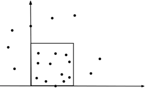
that such axis-parallel unit square may not be unique. In that case, choose one among them and call that axis-parallel unit square as candidate square. Therefore, at most 4n number of candidate squares can be obtained by considering alignments of four different sides for all points in P. Below we describe the pass for computing candidate squares whose bottom sides are passing through a point from P (SeeFigure 1).

Without loss of generality, assume that no two points have the same x- or y-coordinate. Consider two arrays ∆x and ∆y containing the points of P in ascending order of x and y-coordinates respectively.

Let us denote the x-coordinate of the i-th entry of ∆x by xi and similarly the y-coordinate of the i-th

entry of ∆y by yi, 1≤ ≤i n. Coordinates of a generic point p is denoted by

(

x p

( ) ( )

,y p

)

. For a point

p∈P, let left

( )

p denote the minimum entry in ∆x, say q∈P, such that x p

( ) ( )

−x q ≤1.

Observation 1 Given the array ∆x, all intervals x

(

left

( )

pi

)

,x p

( )

i , 1≤ ≤i n can be computed in

[image:2.595.198.435.556.703.2]

linear time.

In a similar way, for a point p∈P, let bottom

( )

p denote the minimum entry in ∆y, say q′∈P, such

that y p

( ) ( )

−y q′ ≤1. Likewise, we define right . , and

( )

top . on the arrays

( )

∆_x and ∆y respectively.

Algorithm for Reporting Candidate Squares

In this section we present sweep line algorithm combined with balanced search tree as data structure for computing candidate squares. Using the points in array ∆x, construct a balanced search tree T with search

key as the x-coordinate values of the points in P. The leaves of T correspond to the ordered points of ∆x.

We attach two positive integral variables  and  with each node of T. Before describing the algorithm in details, we first explain the role of  and . The span I v

( )

corresponding to an internal node v is an interval, generated by the x-coordinates of the left most and right most points at the leaves in the subtree rooted at v. Moreover, span I

( )

µ of the leaf node µ stores the x-coordinate of the point at the leaf node µ of T. Our sweep line algorithm considers two horizontal sweep lines namely bottom sweep line BS and top sweep line TS. Let the current positions of TS and BS be at heights y p

( )

and y q

( )

respectively such that p=top

( )

q and H be the unit horizontal slab determined by BS and TS. In case that the vertical distance between BS and TS is less than unity, shift TS upwards to create a gap between BS and TS as unity. Note that, no additional points are included for such shifting of TS in upward direction.

At the end of processing all points within H , we get the following information by  and . The variable  attached with an internal node v indicates that there exists a subset P′ ⊆

(

P

)

of size  (i.e.,

 stores the count of the set P′) such that each unit square whose bottom, top sides coincide with BS, TS respectively and left boundary within span I v

( )

encloses the subset P′. Observe that these spans I v

( )

are all different for all nodes v. The subsets P′ for nodes along the path from root to a leaf node are all disjoint. Here each node v does not keep P′ explicitly but only its count . The variable  attached with an internal node v indicates that there exists a unit square S whose cardinality is the sum of  values of the ancestor nodes of v plus the  value at node v; bottom and top sides of S are constrained to coincide with BS, TS respectively, the left boundary of S lies within the span I v

( )

. Moreover, the cardinality of S is maximum among all unit squares within the slab H and the left boundary of each such unit square lies within the span of v. We now recursively define  value for an internal node as the sum of its  value and the maximum of  values of its two children-nodes. This recursive definition of  implies that variable  at the root of tree T stores the cardinality of a candidate square whose bottom side is constrained to pass through the point q. This type of integral variables attached to the nodes of segment tree are also used to handle stabbing counting queries [18]. The space requirement for this type of segment tree is linear [18].

In initial step, the variables  and  corresponding to all nodes are initialized with zero and both the sweep lines TS and BS pass through the bottom most point

( )

p1 . Assume that pi is the point

corresponding to the i-th entry in ∆y, 1≤ ≤i n. The algorithm processes all points p p1, 2,,pn in ∆y one

at a time. We also explain the way of capturing information by the variables  and  at the time of processing a point in ∆y, encountered by sweep lines.

The sweep line TS is moved up one point at a time, considering p1 as the first encountered point. For each

point p encountered by the sweep line TS, if the vertical distance of p from the current position of the sweep line BS is less than or equal to unity, T is updated by Increment operation which is described below.

For the interval _x

(

left

( )

p

)

,x p

( )

_, find the split node [18] vsplit in T, that is the least common ancestor

of x

(

left

( )

p

)

and x p

( )

in the balanced search tree T. Search for the leaf node containing left

( )

p on the left subtree rooted at v_split and, while traversing, if we turn left from node v, increment  of the right child of v by one. In case the right child of v is a leaf, increment its  instead of . Similarly, while traversing the right subtree of the split node for searching the leaf node containing p, if we turn right from node v, increment  of the left child of v. Again, in case the left child is a leaf, increment its  instead of . Finally, increase the  values of the leaf nodes containing left

( )

p and p by one. We now recursively update the  value of each internal node in the path from the leaf node containing left

( )

p to the left child of the split node vsplit, as the sum of its  value and the maximum of  values of its two

children-nodes. Then update the  value of each internal node in the path from the leaf containing p to the root of T in similar way. In case x

(

left

( )

p

)

=x p

( )

, we find the leaf node v of T that contains the point p and increment the  value of leaf node v. The subsequent updation of  values associated with the internal nodes of T is same as described earlier.

greater than unity, TS stops advancing to p (i.e., T is not updated by Increment operation for the point p). For the point q on the current position of BS, update T for the point q and report a candidate square with bottom boundary passing though q by the Decrement and Report operations which are explained below. The sweep line BS is then moved up one point at a time. For each point q encountered by the sweep line BS, if the vertical distance between p and q is greater than unity, T is updated by Decrement operation and a candidate square with bottom boundary passing though q is reported by Report operation.

In case that the vertical distance of q from TS becomes smaller than unity, the sweep line BS stops advancing and sweep line TS starts sweeping from its current position. The above process is continued till Report and Decrement operations are done for all the points.

We now describe the Report operation. Let Sq be the candidate square with bottom boundary passing

through the point q. Observe that the number of points enclosed by Sq is equal to the  value at the root

of the tree T. To find a placement of the left boundary of Sq, move from the root of the tree T towards the

leaf, each time picking the child with larger  value. The leaf node thus reached stores the point through which the left boundary of Sq passes. Report Sq along with the number of points inside it.

The Decrement operation is same as Increment operation with the following exception. For the interval

( )

(

left

)

,

( )

x q x q

 

  associated with point q, locate the split node in T. During searching from the split node for the nodes containing left

( )

q and q, instead of incrementing, we decrement ’s and ’s by one as appropriate. The subsequent updation of  values associated with the internal nodes of T is similar to that in the Increment operation.

Theorem 1 Let P be a set of n points in a two dimensional plane. Then all candidate squares for pi∈P,

1≤ ≤i n, can be computed in O n

(

logn time using

)

O n space.

( )

Proof: For a point p, each of Increment, Decrement and Report operation takes O

(

logn

)

time. Since for each point in P, these operations are executed only once, they together take O n

(

logn

)

time. 

Corollary 1 A placement of an axis-parallel unit square enclosing the maximum number of points from P can be computed in O n

(

logn time using

)

O n space.

( )

Proof: Let S* be an axis-parallel unit square enclosing the maximum number of points from P and P′ ⊆P be the set of points enclosed by S*. Note that S* can always be repositioned, without altering the points enclosed by it, so that the extended lines of two adjacent sides of S* pass through two points of P and these two points may not belong to P′. Sometimes the adjacent sides of S* may be passed through same point of P and, in that case, the point is at one corner of S*. Therefore, the maximum cardinality among the set of all possible candidate squares is equal to the cardinality of S*. 

Corollary 2 An axis-parallel rectangle of fixed height and width that encloses the maximum number of points from P, can be placed in O n

(

logn time using

)

O n space.

( )

Proof: Follows directly from Corollary 1. 

Corollary 3 A placement of two disjoint axis-parallel unit squares together enclosing the maximum number of points from P, can be computed in O n

(

logn time using

)

O n space.

( )

Proof: For each point p∈ ∆y, we can compute the cardinality of candidate square whose top boundary is

passing through p in O n

(

logn

)

time. Now, we sweep from bottom to top to generate a subset of ∆y that

reports the maximum cardinality candidate square whose top boundary lies below any point p∈ ∆y. This

sweeping process requires O n

( )

time. 

It is interesting to generalize the maximal enclosing problem using m disjoint axis-parallel unit squares,

2

m> and the problem is known to be NP-hard [19]. A set of m rectangles (squares) on the plane is called m-sliceable if they can be recursively partitioned by

(

m−1

)

horizontal or vertical lines [20]. We now assume there exists m-sliceable axis-parallel squares and propose an algorithm to locate three axis-parallel unit squares which are pairwise disjoint and they together enclose the maximum number of points from P.

Let px_max and py_min be the points with maximum x-coordinates and minimum y-coordinates among the

points in P respectively. Similarly, py_max and px_min be the points with maximum y-coordinates and

minimum x-coordinates among the points in P respectively.

Observe that among these three squares, one square is separated from other two squares by a horizontal or a vertical line. Without loss of generality, assume that the line separating one square from other two squares is vertical (first pass). The other pass where the line separation is horizontal, can be handled in similar manner. Now we are describing the first pass of our proposed algorithm.

and Qi′ respectively; the subset Qi and Qi′ lie on the left and right side of this vertical line. For the position

of the vertical line that passes through the i-point of ∆x, the result in Corollary 3 is used to place a pair of

disjoint squares enclosing the maximum number of points from Qi and the result in Corollary 1 to place a

square that encloses the maximum number of points from Qi′. This triplate of squares is a potential candidate

for position of the vertical line that passes through the i-th entry of ∆x. Observe that the time required to

place these triplet of squares is O(nlogn). Similarly use the result in Corollary 1 to place a square that encloses the maximum number of points from Qi and the result in Corollary 3 to place a pair of disjoint squares

enclosing the maximum number of points from Qi′. This triplate of squares is also a potential candidate for

position of the vertical line that passes through the i-th entry of ∆x. Finally, a triplate of squares that together

enclose greater number of points of P among the two sets of triplet of squares is kept. Now this process is repeated for each position of the vertical line that passes though a point p∈ ∆x. We thus have the following

result.

Corollary 4 Given a set P of n points in the plane, three axis-parallel unit squares which are pairwise disjoint and they together enclose the maximum number of points from P can be placed in

(

2

)

log

O n n time and O n space.

( )

To solve the maximal enclosing problem using m axis-parallel unit squares, if we naively extend this approach then it is interesting to note that the solution would not have a polynomial time complexity in both n and m. Now to solve this problem, we propose an O m n

(

2 5

)

time and O mn

( )

4 space algorithm that uses (i) similar dynamic programming approach as proposed by Mukherjee et al.[21], and (ii) the result in Corollary 1 as a subroutine.

Observe that placing horizontal and vertical partitioning lines among the points of P can generate

( )

4

O n subsets of P. Let P′ ⊆

(

P

)

be the subset of points enclosed by the minimum enclosing rectangle (MER) defined by the points

(

x p

( ) ( )

_i ,y p_k

)

and

(

x p

( )

_j ,y p

( )

_l

)

, i< j and k< as bottom-left and top-right l corners respectively. Given a subset P′ ⊆

(

P

)

, let Count x p

(

( ) ( )

_i ,y p_k ,x p

( )

_j ,y p

( )

_l ,m

)

denote the maximum number of points from P jointly enclosed by m disjoint axis-parallel unit squares placed over the subset P′.

In the first step, we compute Count x p

(

( ) ( )

_i ,y p_k ,x p

( )

_j ,y p

( )

_l ,1

)

for all possible subsets of P using the result in Corollary 1. Subsequently, it computes Count x p

(

( ) ( )

_i ,y p_k ,x p

( )

_j ,y p

( )

_l ,u

)

for all possible subsets of P using the results of the previous steps in similar dynamic programming approach as proposed by Mukherjee et al.[21]. Finally, it reports

(

)

min, min, max, max,

x y x y

Count p p p p m .

In view of the Corollary 1, computation of the first step requires O n

(

5logn

)

. Complexity of subsequent steps, and hence, the over all time complexity of the algorithm is O m n

(

2 5

)

. Corresponding space complexity can also be shown to be _{O mn}

( )

4

. Further details can be found in [21]. We thus have the following result.

Theorem 2 A placement of m sliceable axis-parallel unit squares which are pairwise disjoint and they together enclose the maximum number of points from P can be computed in

(

2 5

)

O m n time using

( )

4

O mn space.

3.

k

-Enclosing Problem

Initially researchers considered the k-enclosing problem for computing a smallest area (perimeter) axis-parallel square or rectangle. Most of the algorithms proposed for k-enclosing problems are efficient when k is small

and become inefficient for large values of k. Segal and Kedem [9] presented an O n

(

+k n k

(

−

)

2

)

time algorithm for finding a smallest area k-enclosing axis-parallel rectangle for large values of k, n 2< <k n.

Matoušek [22] developed O n

(

logn+

(

n k−

)

3n

)

, >0, time algorithm to find a smallest k-enclosing circle that is especially efficient when k is close to n. Given a set P of n points in the plane and an integer k

( )

k ≤n , we consider the problem of computing the minimum area axis-parallel square that encloses at least k points of P for large values of k. A k point enclosing square (rectangle) Sk is said to be a k-square (k-

rectangle) if there does not exist another square (rectangle) having area less than that of Sk and enclosing k

points from P [10].

We use the idea of prune and search technique to solve the optimization problem for finding Sk

(

k>n 2

)

.

points where k and α are the input parameters. In Section 4, we present some preliminary observations and it is shown that the Result in Corollary 1 can be used to solve a decision version of the optimization problem.

4. Preliminaries

Let P=

{

p p1, 2,,pn

}

be the set of n points in the plane. Our objective is to compute k-square Sk.

Without loss of generality, assume that no two points of P have the same x or y coordinates. Let x p

( )

and y p

( )

denote the x-coordinate and the y-coordinate of any point p respectively. The size of a square is represented by the length of it's side. We have the following observation.

Observation 2 At least one pair of opposite sides of S must contain points from k P.

The decision version of this problem can be stated as “given a length α, does there exist a square of size α that encloses at least k points of P?”.

Let Pb, Pt, Pl, Pr and Pf be five subsets of P such that P=Pb   Pt Pl Pr Pf and all the subsets

are not necessarily mutually disjoint. We define Pb and Pt as the set of

(

n k−

)

bottom most and

(

n k−

)

top most points of P respectively; Pl and Pr are the set of

(

n k−

)

left most points and

(

n k−

)

right

most points of P respectively; and Pf = −P P′ where P′ =Pb  Pt Pl Pr.

Note that if k>3 4n then Pf must contain at least one point of P. The following observation follows

from the above definitions.

Observation 3 For k>n 2, S must enclose all the points of k Pf.

Proof: Let p be any point of the set Pf. At least

(

n k−

)

elements are on the right side of p. The

position of p in the left to right ordering of P are at most k. Therefore there are

(

n k− +i

)

number of points of P on the left of p for 0≤ ≤i 2k− −n 1. Consequently at most

(

k−1

)

points are on left of p. Hence right boundary of Sk is on right side of p. Similarly left, top and bottom boundaries of Sk are on left,

top and bottom sides of p respectively. Hence the observation follows.

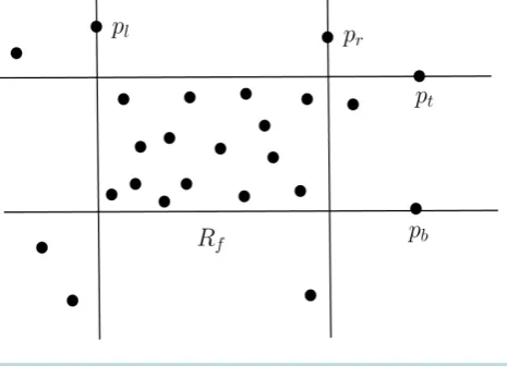
Let Rf be the minimum area axis-parallel rectangle enclosing the point set Pf. Suppose the length of the

longest side of Rf is λ and the left, right, top and bottom boundaries of the rectangle Rf contain the points

l

p , pr, pt and pb respectively (See Figure 2). We define Max-square

( )

α , α λ≥ as an axis-parallel

square of size α that includes the point set Pf and the total number of points enclosed from P is

maximized. It is easy to see that the bottom, top, left and right boundaries of Max-square

( )

α must lie within the ranges _y p

( )

_t −α,y p

( )

_{b } , _y p

( ) ( )

_t ,y p_b +α_ , _x p

( )

_r −α,x p

( )

_l _ and _x p

( ) ( )

_r ,x p_l +α_ respectively.

To locate Max-square

( )

α among the set P′

{

p p p pt, b, l, r

}

, we use sweep line paradigm combined with

binary search tree as data structure in similar way as described in Section 2.1. As earlier, our algorithm makes horizontal and vertical sweeps. Below we briefly describe the algorithm for horizontal sweep to locate

( )

[image:6.595.201.434.540.708.2]

Max-square α whose bottom side is aligned with a point from P. Look for all squares of size α whose bottom and left boundaries are within the range _y p

( )

_t −α,y p

( )

_b _ and _x p

( )

_r −α,x p

( )

_l _ respectively.

Now consider possible positions of the left boundary of Max-square

( )

α within the above mentioned range such that the left boundary or the right boundary passes through a point of P. Notice that all squares with these restrictions include the point set Pf. Therefore the points in the set P′

{

p p p pt, b, l, r

}

are the only points

required to be processed to locate Max-square

( )

α and the number of such points is at most 4

(

n k− +1

)

. This observation leads to the following theorem.

Corollary 5 For given α λ> , the axis-parallel square Max-square

( )

α containing the maximum number of points from P and enclosing point set Pf can be located in O

(

(

n−k

) (

log n−k

)

)

time using O n

( )

space.

5. An Efficient Algorithm to Find

k

-Square for Large Values of

k

In this section, we explain an efficient algorithm to find Sk for large values of

2 n k_> _

 . The result in

Corollary 5 to locate Max-square

( )

α is used as a subroutine to find Sk for

2 n

k> . From Observation 2, we can conclude that either top and bottom sides of Sk contain points of P or left and right sides of Sk contain

points of P. Without loss of generality, assume that top and bottom sides of Sk contain points from P. The

other case where left and right sides of Sk contain points of P, can be handled in similar manner. Let

1, 2, , m

Q= p p  p be an ordering of points of the set P′

{

p p p pl, r, t, b

}

in increasing order of their y

-coordinate values. Consider ∆ to be the list of O

(

(

n−k

)

2

)

vertical distances

(

y p

( )

j −y p

( )

i

)

, j>i for

each pair of points pi and pj∈Q.

Our objective is to find Sk for a given value k such that Max-square

( )

α encloses k points of P and

the value α∈ ∆ is minimized. We iteratively reduce the size of ∆ by prune and search technique without explicitly computing O

(

(

n−k

)

2

)

elements of ∆. Let ∆i represent the list of vertical distances at

th

i iteration. At ith iteration we reduce the size of ∆i by 1 4 . Initially ∆ = ∆0 . Observe that for any pi∈Q,

( )

( )

(

y pj −y pi

)

<

(

y p

( )

j+1 −y p

( )

i

)

for m> >j i. Without loss of generality, let the indices of the points

, ,

l r t

p p p and pb remain same in Q also. Let us denote the set of vertical distances generating ∆ by the

sequences Ψ Ψ1, 2,,Ψb defined as follows.

( ) ( ) (

) ( )

( ) ( )

{

}

( ) ( ) (

) ( )

( ) ( )

{

}

( ) ( ) (

) ( )

( ) ( )

{

}

( ) ( ) (

) ( )

( ) ( )

{

}

1 1 1 1 1

2 2 1 2 2

1 1 , , , , , , , , , , , ,

t t m

t t m

i t i t i m i

b t b t b m b

y p y p y p y p y p y p

y p y p y p y p y p y p

y p y p y p y p y p y p

y p y p y p y p y p y p

+

+

+

+

Ψ = − − −

Ψ = − − −

Ψ = − − −

Ψ = − − −

     

Note that the elements in each sequence Ψi are in nondecreasing order. At th

j iterative step of the algorithm the current search space ∆j is reduced by pruning the Ψi’s. Here, either upper or lower portion of

i

Ψ is pruned. Therefore, each Ψi sequence can be represented by lower and upper indices of the original

sequence. For any point pi∈Q, median element of the corresponding sequence Ψi is

( )

_{1 2}

2

i l l

y p y p_{ + }         −    

where l1 and l2 are the lower and upper indices of the sequence Ψi. We denote the median element of Ψi

as med

( )

Ψi . So computing the median of the sequence of vertical distances corresponding to any point

i

p ∈Q requires only a constant time arithmetic operation on the array indices.

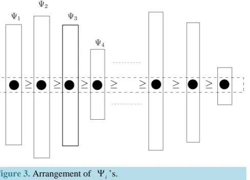
We represent each Ψi as a vertical strip parallel to the y-axis. All the vertical strips (Ψi’s) are arranged

along the x-axis such that med

( )

Ψi 's fall on the x-axis and the median values are in nonincreasing order

along the x-axis (SeeFigure 3). Again the elements of each Ψi are arranged in nondecreasing order parallel

to the y-axis. At initial step of iteration, all medians med

( )

Ψ1 ,med

( )

Ψ2 ,,med

( )

Ψb are in nonincreasing

order. This ordering may change in subsequent iterations due to pruning of Ψi's. Therefore at each iteration, we

need to rearrange Ψi’s such that med

( )

Ψi ’s are in nonincreasing order. Let Ψ Ψ1, 2,,Ψb be an

arrangement of the sequences in ∆j such that med

( )

Ψ ≥1 med

( )

Ψ ≥2 ≥med

( )

Ψb . At th

[image:8.595.195.440.85.261.2]

Figure 3. Arrangement of Ψi’s.

find an index c such that

∑

ci=₁Ψi is half of the size of ∆j. Observe that the size of ∆j is at most 3 4

of the size of ∆j−1. Consider med

( )

Ψc as α and compute Max-square

( )

α . If Max-square

( )

α encloses

at least k points of P, then size of Sk is less than or equal to α and we can ignore the elements in ∆j

greater than med

( )

Ψc . Note that all the med

( )

⋅ values corresponding to Ψ Ψ1, 2,,Ψc−1 are greater than

( )

c

med Ψ . Therefore for each i, 1≤i<c we can delete upper half of Ψi. In case, Max-square

( )

α encloses

less than k points, we similarly delete lower half of each Ψi for c≤ ≤i b. Now continue with the

subsequent iterations until we end up at an iteration, say maxit, such that size of ∆maxit is constant.

Lemma 1 At every iterative step the size of the current solution space is reduced by a factor of 1 4.

Proof: At jth iteration, either we discard upper half of Ψ Ψ1, 2,,Ψc−1 or lower half of Ψ Ψc, c+1,,Ψb.

As the total number of elements in the sequences Ψ Ψ1, 2,,Ψc−1 is 1 2 of size of ∆j, we can discard at

least 1 4 elements of ∆_j. Similar amount of elements is discarded for pruning of lower half.  Now we have the following theorem.

Theorem 3 Given a set P of n points in the plane and an integer 2 n k_> _

 , the smallest area square

enclosing at least k points of P can be computed in

(

(

)

2

(

)

)

log

O n+ n−k n−k time using linear space. Proof: Partitioning the set P to generate subsets P P P Pb, t, l, r and Pf requires O(n) time. Sorting the

points of the sets Pb and Pt with respect to their y-coordinates requires O

(

(

n−k

) (

log n−k

)

)

time. We

do not store the Ψi's explicitly. Instead, for all Ψi's, we maintain an array  whose each element 

[ ]

i

contains the index information l1 and l2 for Ψi at each iteration. So for each Ψi we need only an

additional constant amount of space. Altogether in linear amount of space we can execute our algorithm. Time complexity can be established from the following algorithmic steps at iteration j.

• Computation of med

( )

Ψi for each i requires constant amount of time.

• Sorting the set of all medians med

( )

Ψ1 ,med

( )

Ψ2 ,,med

( )

Ψb takes O

(

(

n−k

) (

log n−k

)

)

time.

• Determining c such that

∑

ci=₁Ψi is half of the size of ∆j, needs O n k

(

−

)

time.

• Computation of Max-square

(

med

( )

Ψ_c

)

takes O

(

(

n−k

) (

log n−k

)

)

time (see Theorem 5).

• We maintain the index structure of the arrays Ψi. This involves updating of l1 and l2 for each Ψi

when half of it's elements are discarded. This step requires constant amount of time for each Ψi.

From Lemma 1, we get that at jth iterative step at least

4 M

elements are discarded where M denotes the

size of ∆j. This leads to the following recurrence relation.

( )

(

)

(

(

) (

)

)

(

(

)

2

(

)

)

3 4 log log

T M =T M +O n−k n−k =O n−k n−k (1) Hence the theorem. 

The technique used to derive the result in Theorem 3 can also compute Sk for all values of k. Hence we

have the following theorem.

Theorem 4 Given a set P of n points in the plane and an integer k

( )

≤n , the smallest area square enclosing at least k points of P can be computed in _{O n}

(

_log2_n

)

Acknowledgments

This research was partially supported by the DST PURSE scheme at University of Kalayni, India.

References

[1] Preparata, F.P. and Shamos, M.I. (1988) Computational Geometry: An Introduction. Springer-Verlag, Berlin.

[2] Chandran, S. and Mount, D. (1992) A Parallel Algorithm for Enclosed and Enclosing Triangles.International Journal of Computational Geometry and Applications, 2, 191-214. http://dx.doi.org/10.1142/S0218195992000123

[3] Toussaint, G.T. (1983) Solving Geometric Problems with the Rotating Calipers. Proceedings of IEEE MELECON, Athens, May 1983, 1-8.

[4] O’Rourke, J. (1985) Finding Minimal Enclosing Boxes. International Journal of Computer and Information Sciences,

14, 183-199. http://dx.doi.org/10.1007/BF00991005

[5] Agarwal, P.K., Sharir, M. and Toledo, S. (1994) Applications of Parametric Searching in Geometric Optimization.

Journal of Algorithms, 17, 292-318. http://dx.doi.org/10.1006/jagm.1994.1038

[6] Aggarwal, A., Imai, H., Katoh, N. and Suri, S. (1991) Finding k Points with Minimum Diameter and Related Problems,

Journal of Algorithms, 12, 38-56. http://dx.doi.org/10.1016/0196-6774(91)90022-Q

[7] Eppstein, D. and Erickson, J. (1994) Iterated Nearest Neighbors and Finding Minimal Polytopes. Discrete and Com-putational Geometry, 11, 321-350. http://dx.doi.org/10.1007/BF02574012

[8] Datta, A., Lenhof, H.P., Schwarz, C. and Smid, M. (1995) Static and Dynamic Algorithms for k-Point Clustering Problems. Journal of Algorithms, 19, 474-503. http://dx.doi.org/10.1006/jagm.1995.1048

[9] Segal, M. and Kedem, K. (1998) Enclosing k Points in Smallest Axis Parallel Rectangle. Information Processing Let-ters, 65, 95-99. http://dx.doi.org/10.1016/S0020-0190(97)00212-3

[10] Das, S., Goswami, P.P. and Nandy, S.C. (2005) Smallest k-Point Enclosing Rectangle and Square of Arbitrary Orienta-tion. Information Processing Letters, 95, 259-266.

[11] Ahn, H., Won, B.S., Demaine, E.D., Demaine, M.L., Kim, S., Korman, M., Reinbacher, I. and Son, W. (2011) Cover-ing Points by Disjoint Boxes with Outliers. Computational Geometry: Theory and Applications, 44, 178-190.

http://dx.doi.org/10.1016/j.comgeo.2010.10.002

[12] Chazelle, B.M. and Lee, D.T. (1986) On a Circle Placement Problem. Computing, 36, 1-16.

http://dx.doi.org/10.1007/BF02238188

[13] Barequet, G., Dickerson, M. and Pau, P. (1997) Translating a Convex Polygon to Contain a Maximum Number of Points. Computational Geometry: Theory and Applicaions, 8, 167-179.

[14] Barequet, G., Briggs, A.J., Dickerson, M.T. and Goodrich, M.T. (1998) Offset-Polygon Annulus Placement Problems.

Computational Geometry: Theory and Applications, 11, 125-141.

[15] Younies, H. and Wesolowsky, G.O. (2004) A Mixed Integer Formulation for Maximal Covering by Inclined Paralleo-grams. European Journal of Operational Research, 159, 83-94.

http://dx.doi.org/10.1016/S0377-2217(03)00389-8

[16] Daz-Báñez, J.M., Seara, C., Antoni, S.J., Urrutia, J. and Ventura, I. (2005) Covering Points Sets with Two Convex Objects. Proceedings of 21st European Workshop on Computational Geometry, 179-182.

[17] Cabello, S., Miguel, D.B.J., Seara, C., Sellares, J.A., Urrutia, J. and Ventura, I. (2008) Covering Point Sets with Two Disjoint Disks or Squares. Computational Geometry: Theory and Applicaions, 40, 195-206.

http://dx.doi.org/10.1016/j.comgeo.2007.10.001

[18] De Berg, M., Van Kreveld, M., Overmars, M. and Schwarzkopf, O. (2000) Computational Geometry—Algorithms and

Applications, Springer-Verlag, Berlin.

[19] Megiddo, N. and Supowit, K.J. (1984) On the Complexity of Some Common Geometric Location Problems. SIAM Journal of Computing, 13, 182-196. http://dx.doi.org/10.1137/0213014

[20] Lengauer, T. (1988) Combinatorial Algorithms for Integrated Circuit Layout, Berlin.

[21] Mukherjee, M. and Chakraborty, K. (2002) A Polynomial-Time Optimization Algorithm for a Rectlinear Partitioning Problem with Applications in VLSI Design Automation. Information Processing Letters, 83, 41-48.

http://dx.doi.org/10.1016/S0020-0190(01)00305-2