Rainfall Prediction using Data Mining Techniques

Rainfall Prediction using Data Mining Techniques

Jyothis Joseph

Department of Computer Science and Engineering. College of Engineering, Kidangoor

Ratheesh T K

Department of Information Technology College of Engineering, Kidangoor

ABSTRACT

Rainfall becomes a significant factor in agricultural countries like India. Rainfall prediction has become one of the most scientifically and technologically challenging problems in the world. A wide variety of rainfall forecast methods are available. There are mainly two approaches to predict rainfall. They are Empirical method and dynamical method. The empirical approach is based on analysis of historical data of the rainfall and its relationship to a variety of atmospheric and oceanic variables over different parts of the world. The most widely used empirical approaches used for climate prediction are regression, artificial neural network, fuzzy logic and group method of data handling. This paper uses data mining techniques such as clustering and classification techniques for rainfall prediction.

Keywords

Data Mining, Clustering, Classification, Artificial Neural Network

1.

INTRODUCTION

A wide variety of rainfall forecast methods are available in India because India is an agricultural country and the success of agriculture depends of rainfall. There are mainly two approaches to predict rainfall. They are Empirical method and dynamical method. The empirical approach is based on analysis of historical data of the rainfall and its relationship to a variety of atmospheric variables. The most widely used empirical approaches used for climate prediction are regression, Artificial Neural Network(ANN), fuzzy logic and group method of data handling. In dynamical approach, predictions are generated by physical models based on systems of equations that predict the evolution of the global climate system in response to initial atmospheric conditions[1].

The objective is to analyze the four months rainfall data i.e. from June to September of a particular region for 9 years because these months are monsoon season for our state Kerala. This paper describes empirical method technique belonging to clustering and classification and approach. ANNs are used to implement these techniques. The artificial neural networks not only analyze the data but also learn from it for future predictions making them suitable for weather forecasting. Neural networks provide a methodology for solving many types of non-linear problems that are difficult to be solved through traditional techniques. Furthermore neural networks are capable of extracting the relationship between inputs and outputs of a process without the physics being explicitly provided. Hence these characteristics of neural networks can be used for the prediction of the weather processes[2]. The input variables given are Temperature, Pressure, Relative humidity, Wind speed, Precipitable water. The technique used for rainfall prediction is classification. In this technique, rainfall values are clustered using subtractive clustering and three classes or states are identified as low, medium and heavy[3]. Data are at 2.5 deg Lat x 2.5 Lon resolution, means the globe is divided into 144 x 73 grids. A daily rainfall data in the period of January 2001 to December

2010 were downloaded from the official website of National Oceanic and Atmospheric Administration (NOAA) maintained by US Department of Commerce. NOAA maintains NCEP/NCAR Reanalysis data. NCEP/NCAR Reanalysis data set is a continually updating gridded data set representing the state of the Earth's atmosphere, incorporating observations and numerical weather prediction model. Downloaded data are between 7.5N-10N Lat and 75E-77.5E Lon that roughly covers the Cochin region.

The paper is organized as follows. After presenting the related works in section 2, section 3 presents the overall architecture of the proposed system. Section 4 discusses Data Collection and preprocessing. The implementation details are discussed in section 5. Results obtained are discussed in section 6. Finally, the paper is concluded in section 7.

2.

RELATED WORK

Volume 83 – No 8, December 2013

12

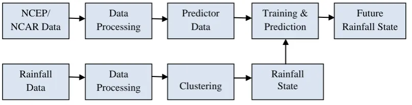
Fig 1: System Architecture

In the paper [5] ANNs are used to obtain a forecasting model for the daily rainfall of Mashhad’s synoptic station in Iran. This is due to the intelligent capability of the neural networks in the extraction of the features of the systems, even in the cases that there is not much information about the system dynamics. Three-layer feed-forward perceptron network with back propagation algorithm is used to implement the model. It is assumed that the network does not have any a priori knowledge about the problem. Therefore, the network must be firstly trained with repeated sets of input patterns. During the training process, the error between the desired output and the calculated output is propagated back through the network, hence is called back propagation algorithm. In the paper [6] ANNs have been extensively used in these days in various aspects of science and engineering because of its ability to model both linear and non-linear systems without the need to make assumptions as are implicit in most traditional statistical approaches. ANN has been an aggressive model over the simple linear regression model. Artificial neural network is one of the most widely used supervised techniques of data mining. In this paper we used the back propagation neural network model for predicting the rainfall based on humidity, dew point and pressure in the country India. Two-Third of the data was used for training and One-third for testing .The number of training and testing patterns are 250 training and 120 testing

The paper [7] describes two rainfall prediction models were developed and implemented in Alexandria, Egypt. These models are ANN model and Multi Regression MLR model. A Feed Forward Neural Network (FFNN) model was developed and implemented to predict the rainfall on yearly and monthly basis. In order to evaluate the incomes of both models, statistical parameters were used to make the comparison between the two models. These parameters include the Root Mean Square Error RMSE, Mean Absolute Error MAE, Coefficient Of Correlation CC and BIAS. The paper [8] describes how neural networks can be used as a useful statistical tool for nonparametric regression. In this paper, a methodology is developed for nonparametric regression within the Bayesian paradigm. Here feed-forward networks with one hidden layer of nodes with logistic activation functions and with one linear output are used. Neural networks are a class of nonparametric regression models that originated as an attempt to model the act of thinking by modeling neurons in the brain. The underlying statistical idea of a neural network is that it uses logistic functions to form a basis over the space of continuous functions, with each hidden node corresponding to a basis function. With an infinite number of hidden nodes, one can match any function arbitrarily closely. In practice, only a finite number of hidden units are used, forming an approximation to the best regression function.

The paper [9] describes K-means clustering; Fuzzy C means clustering, Mountain clustering, and Subtractive clustering. The technique is Mountain clustering, proposed by Yager and Filev .This technique calculates a mountain function (density function) at every possible position in the data space, and chooses the position with the greatest density value as the center of the first cluster. It then destructs the effect of the first cluster mountain function and finds the second cluster center. This process is repeated until the desired number of clusters has been found. The fourth technique is Subtractive clustering, proposed by Chiu. This technique is similar to mountain clustering, except that instead of calculating the density function at every possible position in the data space, it uses the positions of the data points to calculate the density function, thus reducing the number of calculations significantly.

3.

PROPOSED ARCHITECTURE

The overall architecture of the system is shown in Fig 1.

The NCEP/NCAR datasets are preprocessed using prestd function. It is fed as inputs for training. The rainfall values are clustered using subtractive clustering and the rainfall states identified as low, medium, heavy and given as outputs for training. Separating data into training and testing sets is an important part of evaluating data mining models. When we separate a data set into a training set and testing set, most of the data is used for training, and a smaller portion of the data is used for testing. Here 80% of the dataset is used for training and the remaining 20 % for testing.

4.

DATA

COLLECTION

AND

PREPROCESSING

Datasets for rainfall prediction downloaded from official website of National Oceanic and Atmospheric Administration (NOAA) maintained by US Department of Commerce. The NOAA is a scientific agency within the United States Department of Commerce focused on the conditions of the oceans and the atmosphere. NOAA warns of dangerous weather, charts seas and skies, guides the use and protection of ocean and coastal resources, and conducts research to improve understanding and stewardship of the environment.

NOAA maintains NCEP/NCAR Reanalysis data. The NCEP/NCAR Reanalysis data set is a continually updating gridded data set representing the state of the Earth's atmosphere, incorporating observations and numerical weather prediction (NWP) model output dating back to 1948. It is a joint product from the National Centers for Environmental Prediction (NCEP) and the National Center for Atmospheric Research (NCAR). The National Centers for Environmental Prediction (NCEP) and National Center for Atmospheric Research (NCAR) have cooperated in a project called reanalysis to produce a retroactive record of more than 50 years of global analyses of atmospheric fields in support of NCEP/

NCAR Data

Data Processing

Predictor Data

Training & Prediction

Future Rainfall State

Rainfall Data

Data

Processing Clustering

the needs of the research and climate monitoring communities. These data were then quality controlled and assimilated with a data assimilation system kept unchanged over the reanalysis period. This eliminated perceived climate jumps associated with changes in the operational (real time) data assimilation system, although the reanalysis is still affected by changes in the observing systems.

The National Centers for Environmental Prediction (NCEP) and the National Center for Atmospheric Research (NCAR) have accomplished different re-analysis projects which aim on the generation of global data sets for a long time period for different atmospheric parameters. The re-analysis is created with a model similar to the one used for weather forecasts. This model is initialized with measured data from different sources, including observations from weather stations, ship, aircraft, and satellite. Using one model for the whole re-analysis period generates homogeneous data that can be used for long term studies. NCEP/NCAR has produced several re-analyses that are described on their web-page. This free data set is updated continuously and has therefore many users worldwide.

4.1

Feature Extraction

It is the technique of selecting a subset of relevant features for building robust learning models. Many features like Temperature, Evaporation, Wind Speed, Terrain features, Height from sea level, humidity, Precipitable water affects the rainfall .Out of it, the most relevant five features are considered in this paper. The following are the features selected.

4.1.1

Relative Humidity

Relative humidity is a term used to describe the amount of water vapor in a mixture of air and water vapor. It is defined as the ratio of the partial pressure of water vapor in the air-water mixture to the saturated vapor pressure of air-water at the prescribed temperature. The relative humidity of air depends not only on temperature but also on the pressure of the system of interest. Relative humidity is often used instead of absolute humidity in situations where the rate of water evaporation is important, as it takes into account the variation in saturated vapor pressure.

4.1.2

Pressure

Air pressure varies over time and from place to place and these temporal differences are usually caused by the temperature of the air. Cool air is denser (heavier) than warm air. Warm air is less dense (lighter) than cool air and will therefore rise above it. Areas of high pressure can be caused when cool air is sinking and pressing on the ground. At this time, the weather is usually dry and clear. In contrast, when warm air rises, it causes a region of low pressure. With low pressure, the weather is often wet and cloudy.

4.1.3

Temperature

Atmospheric temperature is a measure of temperature at different levels of the Earth's atmosphere. It is governed by many factors, including incoming solar radiation, humidity and altitude. Air temperature is the intensity aspect of sun's energy that strikes the earth's surface. Because the amount of energy from the sun reaching the earth varies from day to day, from season to season, and from latitude to latitude, temperatures also vary. The earth as a whole receives a constant flow of radiant short-wave energy from the sun. The earth also radiates long-wave energy to space. During the day, the flow of short-wave radiation absorbed exceeds long -wave energy emitted, and the surface temperature increases.

4.1.4

Precipitable Water

Precipitable water is the depth of water in a column of the atmosphere if all the water in that column were precipitated as rain. The total atmospheric water vapor contained in a vertical column of unit cross-sectional area extending between any two specified levels, commonly expressed in terms of the height to which that water substance would stand if completely condensed and collected in a vessel of the same unit cross section.

4.1.5

Wind Speed

Wind is the flow of gases on a large scale. On Earth, wind consists of the bulk movement of air. Wind is caused by differences in pressure. When a difference in pressure exists, the air is accelerated from higher to lower pressure. Wind speed is affected by a number of factors and situations, operating on varying scales . These include the pressure gradient, Rossby waves and jet streams, and local weather conditions. There are also links to be found between wind speed and wind direction, notably with the pressure gradient and surfaces over which the air is found.

4.2

Data Processing

Downloaded datasets are in NetCDF (nc) format. NetCDF (Network Common Data Form) is a set of software libraries and self-describing, machine-independent data formats that support the creation, access, and sharing of array-oriented scientific data. Two packages are used to convert NC Format to ASCII. They are NetCDF & FAN. Unidata's NetCDF package includes ncdump, which is used to display the metadata from a NetCDF file. ncdump -h filename will display only the header information, without any of the actual data. Data is stored in the NetCDF files in 2D arrays. To extract the data, we need to know the name of the variable and the array indices of the grid cell we want to extract. Give nc2text the filename, the variable, and the indices redirecting the output to a text file Harvey Davies' FAN (File Array Notation) is an array-oriented language for identifying data items in files for the purpose of extraction or modification. In this paper, the utility nc2text which is available in FAN is used to convert netCDF data to plain text.

5.

IMPLEMENTATION

Clustering is the process of organizing objects into groups whose members are similar in some way. A cluster is therefore a collection of objects which are similar between them and are dissimilar to the objects belonging to other clusters. Clustering can be considered the most important unsupervised learning problem. In this paper subtractive clustering is used. Subtractive clustering is a fast, one-pass algorithm for estimating the number of clusters and the cluster centers in a set of data. This means that the computation is now proportional to the problem size instead of the problem dimension. However, the actual cluster centers are not necessarily located at one of the data points, but in most cases it is a good approximation, especially with the reduced computation this approach introduces. The subtractive clustering method assumes each data point is a potential cluster center and calculates a measure of the likelihood that each data point would define the cluster center, based on the density of surrounding data points.

Volume 83 – No 8, December 2013

14 neurons, these two layers connect the network to the outside

world. In addition to these two layers, the multilayer perceptron usually has one or more layers of hidden neurons, which are so called because these neurons are not directly accessible. The hidden neurons extract important features contained in the input data. Feed forward networks often have one or more hidden layers of sigmoid neurons followed by an output layer of linear neurons. Multiple layers of neurons with nonlinear transfer functions allow the network to learn nonlinear relationships between input and output vectors.

Neural network training can be made more efficient if certain preprocessing steps are performed on the network inputs and targets. In this paper preprocessing and post processing is done using prestd, poststd & trastd. It normalizes the inputs and targets so that they will have zero mean and unity standard deviation. The following code illustrates the use of prestd.

[pn,meanp,stdp,tn,meant,stdt] = prestd(p,t)

The original network inputs and targets are given in the matrices p and t. The normalized inputs and targets, pn and tn, that are returned will have zero means and unity standard deviation. The vectors meanp and stdp contain the mean and standard deviations of the original inputs, and the vectors meant and stdt contain the means and standard deviations of the original targets. After the network has been trained, these vectors should be used to transform any future inputs that are applied to the network. They effectively become a part of the network, just like the network weights and biases. If prestd is used to scale both the inputs and targets, then the output of the network is trained to produce outputs with zero mean and unity standard deviation. If we want to convert these outputs back into the same units that were used for the original targets, then we should use the routine poststd. In the following code we simulate the network that was trained in the previous code, and then convert the network output back into the original units.

an = sim(net,pn)

a = poststd(an,meant,stdt)

The network output an corresponds to the normalized targets tn. The un-normalized network output a is in the same units as the original targets t. If prestd is used to preprocess the training set data, then whenever the trained network is used with new inputs, they should be preprocessed with the means and standard deviations that were computed for the training set. In the following code, we apply a new set of inputs to the network we have already trained.

pnewn = trastd(pnew,meanp,stdp)

anewn = sim(net,pnewn)

anew = poststd(anewn,meant,stdt)

The determination of appropriate number of hidden layer neuron is one of the most critical tasks in neural network design. Unlike the input and output layers, one starts with no prior knowledge as to the number of hidden layer neurons. A network with too few hidden nodes would be incapable of differentiating between complex patterns leading to only a linear estimate of the actual trend. In contrast, if the network has too many hidden nodes it will follow the noise in the data due to over-parameterization leading to poor generalization for untrained data. With increasing number of neurons, training becomes excessively time-consuming. The most popular approach to finding the optimal number of hidden

layer neurons is by trial and error. In this paper FFNN consisted of one input layer, one hidden layer with 50 nodes and one output layer.

The activation function is a function used to transform the activation level of a unit or rather a neuron into an output signal. Typically, activation functions have a “squashing” effect; they contain the output within a range. There are many activation functions that can be applied to neural networks. In this paper, the activation function used in the hidden layer is the Tan-Sigmoid transform function, or tan-sig function. The activation function used in the output layer is the linear transform function, or purelin function. It is defined as follows f(x)=x. For training, trainbr function is used in this paper. In this framework, the weights and biases of the network are assumed to be random variables with specified distributions. The regularization parameters are related to the unknown variances associated with these distributions. We can then estimate these parameters using statistical techniques. Bayesian regularization has been implemented in the function trainbr . When using trainbr , it is important to let the algorithm run until the effective number of parameters has converged. The training might stop with the message "Maximum MU reached." This is typical, and is a good indication that the algorithm has truly converged. When the data set is small and you are training function approximation networks, Bayesian regularization provides better generalization performance. This is because Bayesian regularization does not require that a validation data set be separate from the training data set; it uses all the data.

6.

RESULTS

Applying subtractive clustering, the optimum numbers of clusters are obtained as 3.The rainfall values are categorized as low, medium & heavy. The classifier model has been evaluated against a confusion matrix and the following results have been obtained. Confusion matrix is a matrix in which each column of the matrix represents the instances in a predicted class, while each row represents the instances in an actual class. True Positives (TP), True Negative (TN), False Negative (FN), false Positive (FP) are the four different possible outcomes of the prediction of the confusion matrix. A false positive is when the outcome is incorrectly classified as positive when it is in fact negative. A false negative is when the outcome is incorrectly classified as negative when it is in fact positive. True positives and true negatives are obviously correct classifications.

Accuracy is the overall correctness of the model and is calculated as the sum of correct classifications divided by the total number of classifications. Accuracy = (TP + TN)/ (TP + TN + FP + FN). Precision is a measure of the accuracy provided that a specific class has been predicted. It is defined as Precision = TP/ (TP + FP) where TP and FP are the numbers of true positive and false positive predictions for the considered class. Recall is a measure of the ability of a prediction model to select instances of a certain class from a data set. It is also called sensitivity, and corresponds to the true positive rate. It is defined by the formula Recall = Sensitivity = TP / (TP + FN) where TP and FN are the numbers of true positive and false negative predictions for the considered class.

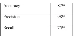
Table 1. Performance Measures

Accuracy 87%

Precision 98%

Recall 75%

7.

CONCLUSION

Rainfall prediction has been one of the most scientifically and technologically challenging task in the climate dynamics and climate prediction theory around the world in the last century. This paper applies neural network for rainfall prediction. In this paper two methods such as classification and clustering are implemented. The neural network Bayesian regularization has been applied in the implementation.

8.

REFERENCES

[1] M.Kannan, S.Prabhakaran, P.Ramachandran “Rainfall Forecasting Using Data Mining Technique” International Journal of Engineering and Technology Vol.2 (6), 2010, pp. 397-401.

[2] Jasmeen Gill, Baljeet Singh and Shaminder Singh, "Training Back Propagation Neural Networks with Genetic Algorithm for Weather Forecasting”, IEEE 8th International symposium on intelligent systems and informatics Serbia, 2010.

[3] Sumi S.Monira, Zaman M.Faisal,H.Hirose ”Comparison of Artificially Intelligent Methods in Short Term Rainfall Forecast” the 13th International Conference on Computer And Information Technology (ICCIT 2010) , vol.PID728, 2010.12.

[4] S. Kannan , Subimal Ghosh, ”Prediction of daily rainfall state in a river basin using statistical downscaling from GCM output, Stochastic Environmental Research and Risk Assessment. May 2011, Volume 25, Issue 4, pp 457-474.

[5] Najmeh Khalili , Saeed Reza Khodashenas et al. “Daily Rainfall Forecasting for Mashhad Synoptic Station using Artificial Neural Networks” 2011 International Conference on Environmental and Computer Science IPCBEE vol.19(2011) © (2011) IACSIT Press, Singapore.

[6] Enireddy.Vamsidhar K.V.S.R.P.Varma et al. “Prediction of Rainfall Using Backpropagation Neural Network Model” (IJCSE) International Journal on Computer Science and Engineering Vol. 02, No. 04, 2010, pp. 1119-1121.

[7] A. Elshafie, A. Shehata,Hasan G. El Mazoghi et al. “Artificial neural network technique for rainfall forecasting applied to Alexandria, Egypt” International Journal of the Physical Sciences Vol. 6(6), pp. 1306– 1316, 18 March, 2011 ISSN 1992-1950 ©2011 Academic Journals.

[8] Herbert K. H. Lee ISDS, Duke University, “A Framework for Nonparametric Regression Using Neural Networks”, Technical Report 00-32, Duke University, Institute of Statistics and Decision Sciences.