Mapping spatial variability of soil physical properties for site specific management

(1)

Mapping spatial variability of soil physical properties for site-specific

management

Henry Oppong Tuffour

1,

**_{*, Awudu Abubakari}**

1

_{, Janvier Bigabwa Bashagaluke}

1,2

_{, Ebenezer}

Djaney Djagbletey

1,3

1_{Department of Crop and Soil Sciences, Kwame Nkrumah University of Science and Technology, Kumasi, Ghana}

2_{Department of Soil Science, Faculty of Agriculture, Catholic University of Bukavu, DR Congo}

3_{Ghana Forestry Commission, Cape Coast}

---*---Abstract -**

Description of the spatial patterns of soil

properties at the field or watershed scale is very important for site-specific soil and crop management, and environmental modelling. The study was conducted to determine the spatial distribution patterns of soil physical properties in an agricultural field in the surface (0-20 cm) and subsurface (20-40 cm) layers. Descriptive statistics and geostatistics were used to describe the amount and form of variability and spatial distribution patterns of the soil physical properties in the field using GraphPad Prism version 6.0 and GS+ 9.0, respectively. The descriptive statistics revealed that the soil properties exhibited weak to higher variations in both layers cross the field, with aggregate stability being the most reliable soil physical property in the field. The spatial distribution model, spatial dependence levels and spatial distribution maps showed remarkable variations in both layers across the field. The significance of semivariogram modelling for the subsequent interpolation was proven to be an effective tool for delineation of management zones for site-specific soil management.

Key Words: Autocorrelation, kriging, semivariogram, site-specific soil management, spatial dependence

1. INTRODUCTION

Spatial variability of soil physical properties within or among agricultural fields is inherent in nature due to both geologic and pedologic factors of soil formation. However, management practices such as tillage, irrigation, and fertilizer application may also induce variability within the field and may further interact with each other across different spatial and temporal scales, and are further modified locally by erosion and deposition processes [1]. Spatial properties of field soils, thus, vary in a complex manner, especially in arid and semi-arid environments where this phenomenon affects the quality and production of crops, hydrologic responses and transport of herbicides to surface and/or groundwater. [2, 3]. Traditionally, researchers have attempted to remove spatial variability by blocking and/or statistical averaging procedures. However, these attempts have often resulted in the failure to understand the spatial interdependence of the soil properties. An appropriate understanding of the spatial variation of soil properties and the relationships between them is needed to scale up measured soil properties, and

model soil processes for precision farming/forestry and environmental modelling. The study was, therefore conducted to analyze the extent of spatial variability in selected soil physical properties.

2. MATERIALS AND METHODS

2.1. Site location and characteristics

The study was conducted at the Plantations Section of the Department of Crop and Soil Sciences, of the Kwame Nkrumah University of Science and Technology, Kumasi, Ghana. The experimental field was located in an uprooted oil palm (Elaies guineensis) field, where spatial variability was predictable due to the variable biological activity and the presence of dead root channels and burrows of soil animals [4]. The area is within the semi-deciduous forest zone of Ghana. It is subjected to two growing seasons (a major and a minor season) with a bimodal rainfall pattern. The major season starts in May and is interrupted by a dry period in August. The minor season starts from September to November. Annual rainfall is about 1375 mm. Annual temperature ranges from 25 – 35°_{C. The dominant soil is the}

Kumasi series described as Plinthi Ferric Acrisol [5] or Typic Plinthustult [6].

(2)

2.3. Soil sampling and analyses

Cylindrical core samplers of 8.1 cm diameter and 20 cm length were used for the collection of soil samples. The collected samples were used for the analyses of particle size distribution using the hydrometer method [9], volumetric moisture content [10], bulk density and total porosity [11], and aggregate stability [12].

2.4. Data analyses

Measured variables in the data set were analyzed in two distinct stages. First, the descriptive statistics including the minimum, maximum, mean, coefficient of variation (CV), skewness and kurtosis were estimated for each property at each depth using GraphPad Prism version 6.0. Characterization of CV was conducted as described by Tuffour et al. [4] and Wilding [13]. The symmetry and peakedness of the data distribution based on the coefficients of skewness and kurtosis were used to determine the order of data distribution in the field. However, since it was expected that small variations could arise and produce a chance fluctuation of skewness and kurtosis measures from zero (Normal distribution), each variable was validated to determine the type of distribution from which the samples were taken using the D’Agostino-Pearson “Omnibus K2” test [4, 14].

Geostatistical calculations and interpolations were used to describe the spatial dependence of each soil property using GS+ 9.0 software. Regarding the fact that normality of distribution is not a pre-requisite of geostatistical processing the original data set was processed without any transformation [4, 15]. Spatial variability was evaluated using the semivariogram for both isotropical and anisotropical orientations. The anisotropic evaluations were performed in four different directions (0°_{, 45}°_{, 90}°_{and 135}°₎

with a tolerance of 22.5° to determine whether semivariogram functions depended on sampling orientation and direction (i.e., they were anisotropic) or not (i.e., they were isotropic), and the commonly used models were fitted for each soil property [4]. The best fit model was chosen using the Least Squares method and the spatial dependence (SD) was defined using the nugget/sill ratio [4, 16]. Surface maps of the soil properties were prepared using semivariogram parameters through ordinary Kriging and prediction performance was assessed by cross-validation [4].

3. RESULTS AND DISCUSSIONS

3.1. Descriptive statistics

The spot-to-spot variations in the soil physical properties as observed from the measured descriptive statistical values are presented in Table 1. The results showed significant differences between the mean values at both sampling depths across the field. These variations could be ascribed to a combination of factors including experimental errors, and temporal and spatial variations.

3.1.1. Variation in particle size distribution

The top layer showed different textural classes of loamy sand, sandy loam and sandy clay loam. Except for two spots with sand, and sandy clay texture each, soils in the subsurface were dominantly sandy loam and loamy sand textured. The coefficients of variation for sand content in both layers were classified as low, whereas those of silt and clay were classified as very high, with the sub surface layer showing higher variability than the upper layer. Among the primary soil particles, the mean sand and silt contents were slightly lower in the subsurface layer than in the surface layer, whereas the mean clay content was higher in the subsurface layer than in the surface layer. The high CV values of silt and clay could have resulted from the previous land use system and soil management strategies in the field.

Although studies by Santra et al. [17] showed that soil mixing due to tillage operations can result in little variation of particle size distribution in the surface layer than the subsurface layer, the modified minimum tillage method employed in the land preparation process in this study yielded similar results, except for clay content. The low variability of particle size fractions at the surface layer as compared to the subsurface layer could, thus, be attributed to the susceptibility of the soil aggregates to erosion and deposition of soil particles from one spot to another in the field. This is because these processes tend to distribute the soil particles, somehow, uniformly in the field. Additionally, the eluviation-illuviation processes due to downward movement of water through the soil may have resulted in the deposition of fine-grained particles (especially clay) within the underlying layers beneath the soil surface. The differences in the influence of parent materials (i.e. resistance or susceptibility to weathering) may also have affected the distribution of soil particles in the field.

Silt and clay fractions gave positive and highest kurtosis in the surface layer and subsurface layers, respectively. The kurtosis value for sand in the surface layer, although positive, showed a normal (mesokurtic) distribution, not only because it was closer to zero, but also established from the K2 test. On the other hand, the kurtosis values for the different soil fractions in subsurface layer were too tall or slender than a normal distribution. The results also showed positive skewness for clay and silt contents, and negative skewness for sand content in both layers. Similarly, even though the coefficient of skewness for sand in the surface layer extended toward the left, showing a shift from normal distribution, the K2 test revealed it was normally distributed across the field. This indicates that the variation of sand content in the surface layer as revealed by the coefficient of variability could be due to chance.

3.1.2. Variation in soil structure indicators

(3)

were highly variable in the surface layer than the subsurface layer, however, the variation in both layers were categorized as weak as revealed by the coefficients of variability [4,13]. Similarly, values of aggregate stability in both layers, although very low, were found to be weakly variable, indicating an almost homogeneous aggregate stability across the field. This could be accredited to the high susceptibility of the soil aggregates to erosion and depositional events occurring at the soil surface, causing an almost evenly distribution of the soil aggregates at the soil surface. On the other hand, the differences in organic carbon [4] and moisture contents in both layers could be accountable for the unequal distribution of aggregate stability with depth. Thus, aggregate stability was described as the most reliable soil property in the field, implying that any single value from any spot in the field for a particular layer could be used to represent the whole field for that particular layer. The low aggregate stability observed within both layers could be attributed to the previous tillage operations (ploughing and harrowing), which caused significant disturbance to the surface and subsurface soil structure, organic matter and clay contents resulting in considerable amounts of compaction as evidenced by the high bulk density and low total porosity. This further resulted in the destruction of soil aggregates [18]. The relatively high aggregate stability observed in the surface layer than the subsurface layer could have resulted from the accumulation of organic residues (high organic carbon content) on the soil surface [4].

With regards to the frequency distribution, the kurtosis values for aggregate stability in both layers were negative and platykurtic (i.e., flat). However, the coefficients of skewness were zero, signifying that aggregate stability was normally distributed across the field in both layers. Except for one outlier, which caused a tall peaked distribution, the distribution of aggregate stability of the surface layer was almost uniform and flat across the field as evidenced by the coefficient of variation (0.16%), which was the weakest for the entire data set in the study. The K2 test values further showed that aggregate stability was normally distributed within the field in both the surface and subsurface layers. For bulk density and total porosity in the surface layer, the coefficients of kurtosis were positive and close to zero, which described a leptokurtic distribution. Moreover, the coefficients of skewness for the properties indicated a distribution towards the more negative values, however, the outcome of the K2 test (2.88), which was the same for both properties described a normal distribution for both parameters. The coefficient of skewness also showed a distribution more toward the positive direction.

3.1.3. Variation in soil moisture content

The soil moisture values (i.e. volumetric moisture content) determined in the different locations and depths were used to describe the spatial variability of soil moisture content in the field. Although the spot-to-spot measured values ranged

from 6.64 – 17.52% and 7.78 – 17.44%, the average values were 11.33% and 12.68% for the surface and subsurface layers, respectively. From the coefficients of variation, it was realized that soil moisture was varied moderately across the field. The variability of soil moisture as observed in this study could have been influenced by both static (topography and soil properties) and dynamic (precipitation and initial moisture content) variables [19, 20], which may be responsible for the different moisture patterns during wetting, draining and drying periods [21]. In addition, K2 test value, as well as the coefficients of kurtosis (negative) and skewness (positive) all showed that soil moisture content was normally distributed in the field. The observed variability of soil water content may have very important impact on rainfall-infiltration/runoff/erosion processes, especially under high rainfall conditions, and also result in spatial variability of available water for crop growth, which is identified as one of the major reasons for the variations in crop growth and productivity in an area.

(4)

[image:4.595.32.570.115.379.2]

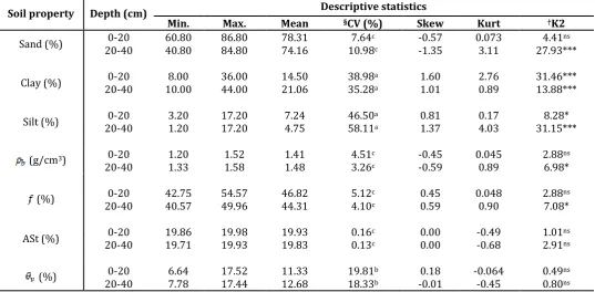
Table 1: Summary of descriptive statistics of measured soil physical properties

Soil property Depth (cm) Descriptive statistics

Min. Max. Mean §_{CV (%)} _Skew _Kurt †_K2 Sand (%) _20-400-20 _40.8060.80 86.80 _84.80 78.31 _74.16 _10.987.64c_c -0.57 _-1.35 0.073 _3.11 _27.93***4.41ns

Clay (%) _20-400-20 _10.008.00 36.00 _44.00 _21.0614.50 38.98_35.28a_a _1.011.60 _0.892.76 31.46*** _13.88***

Silt (%) _20-400-20 3.20 _1.20 17.20 _17.20 _4.757.24 46.50_58.11a_a _1.370.81 _4.030.17 _31.15***8.28*

(g/cm3₎ 0-20 1.20 1.52 1.41 4.51c -0.45 0.045 2.88ns

20-40 1.33 1.58 1.48 3.26c _-0.59 _0.89 _6.98*

(%) 0-20 42.75 54.57 46.82 5.12c 0.45 0.048 2.88ns

20-40 40.57 49.96 44.31 4.10c _0.59 _0.90 _7.08*

ASt (%) _20-400-20 19.86 _19.71 19.98 _19.93 19.93 _19.83 _0.130.16c_c 0.00 _0.00 _-0.68-0.49 _2.911.01ns_ns

(%) 0-20 6.64 17.52 11.33 19.81b 0.18 -0.064 0.49ns

20-40 7.78 17.44 12.68 18.33b _-0.01 _-0.45 _0.80ns

= Bulk density; = Total porosity; = Volumetric moisture content;ASt (%) = Aggregate stability;Min. = Minimum parameter value; Max. = Maximum parameter value; §_{CV = Coefficient of variation (a, b, c = very high, moderate and weak}

variations, respectively); †_{K2 = Omnibus Normality Test (***, **, *, ns = highly significant, moderately significant, significant and}

(5)

3.2. Spatial structure and attributes

Spatial structure analyses using semivariograms and autocorrelograms revealed significant spatial variability of the soil properties across the field. The best-fit models and model parameters are presented in Table 2. Among the different theoretical models tested, exponential model was found to be the best-fit in most cases. The observed differences in spatial relationships for the soil properties were attributed to both intrinsic and extrinsic factors of soil formation. Isotropic models were selected as ideal representation of semivariograms for the soil properties since the best-fit models were the same in all directions. The behaviour of the soil properties in space is visually presented in Figures 1-3. Except for silt content in the subsurface, and aggregate stability and porosity in the surface layer, which were best-fitted by linear model (i.e. pure nugget effect or absence of spatial correlation), all the other parameters in both layers were best-fitted by the transitive semivariogram models (i.e. Gaussian, Exponential and Spherical models), indicating variations in the spatial correlation structure with the lag. The results also revealed that as lag increased, correlations dropped either gradually or rapidly to zero, and then fluctuated about or remained at it, which suggests that the correlated values had dependent and/or interdependent relationships.

Class ratios to identify the distinctive classes of spatial dependence (i.e. autocorrelation) for the resulting semivariograms indicated the existence of weak to strong spatial dependence for the soil properties. This implies that at greater separation distance than the range, sampling points would not be spatially correlated, which would have great implications on sampling design. Thus, separation distances should be shorter than the range in order to properly understand the spatial distribution pattern of the given property. As a result, Balansundram et al. [22] have recommended that sampling points should be spaced 0.25 – 0.50 of the range. Therefore, in view of the range, sampling spacing should be closer for shorter ranges than those with longer ranges.

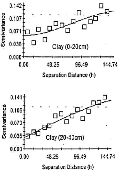
3.2.1. Spatial structure of particle size distribution

The best-fit semivariogram models for the various soil particles are presented in Figures 1a- c. Considering the surface layer the models were exponential, Gaussian and spherical for sand, clay and silt contents, respectively, whereas, in the subsurface layer, Gaussian, spherical and linear models best-fitted the soil particles in the same respective order as in the surface layer. The soil particles also expressed low positive non-zero nugget values, which could be explained as due to minimum sampling errors, sampling intensity and data recording, short range variability, and random and inherent variability. From the analyses, silt content in the surface layer displayed a well-defined spatial structure (clear characteristic sill and range) with important, but not too large nugget semivariance typical of a spherical model.

Sand and clay contents in the surface and subsurface layers, on the other hand, displayed clear nugget and sill values, but gradually approached the range, specifying an exponential model. Contrarily, sand and clay in the subsurface and surface layers, respectively, were best-fitted by a Gaussian model, owing to the smooth variation with small nugget semivariance as compared to the spatially dependent random variation. For silt content in the subsurface layer, the property was found to vary at all scales, hence it was best-fitted by a linear model. With regards to the range of influence, defined as the maximum distance of spatial dependence between sample pairs, the results showed that the best sampling distance alternated within 165.76 – 415.80 m for sand, 188.62 – 216.90 m for clay and 11.70 m for silt contents. This implies that any pair of particle size values with a lag greater than 415.80, 216.90 and 11.70 m for sand, clay and silt, respectively will be spatially independent. Thus, sampling for the analysis of soil texture should not exceed a maximum distance of 416 m, and this will very much depend on the sampling interval, which greatly influences the semivariogram range [23].

(6)

[image:6.595.52.254.88.411.2]

[image:6.595.327.546.115.418.2]

Figure 1a: Best-fitted isotropic semivariogram for sand content for the surface and subsurface layers

[image:6.595.54.243.449.724.2]

Figure 1b: Best-fitted isotropic semivariogram for clay content for the surface and subsurface layers

Figure 1c: Best-fitted isotropic semivariogram for silt content for the surface and subsurface layers

(7)

[image:7.595.320.527.123.421.2]

40 m area with 10 x 5 m sampling intervals used in this study.

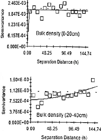
[image:7.595.51.265.162.458.2]

Figure 2a: Best-fitted isotropic semivariogram for bulk density for the surface and subsurface layers

(8)

[image:8.595.49.542.53.429.2]

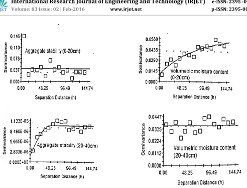
Figure 2c: Best-fitted isotropic semivariogram for aggregate stability for the surface and subsurface

layers

3.2.3. Spatial structure of moisture content

The semivariogram functions for volumetric moisture content were exponential and spherical the surface and subsurface layers, respectively as shown in Figure 3. In the surface layer, a fairly higher nugget and sill, and higher range were observed in contrast to the subsurface layer, with exception of the range. These observations were indicative of small estimated errors, which occurred in the subsurface layer. The range in the subsurface layer also showed that moisture content was spatially correlated at a very short distance, which implied that sampling for moisture measurements should be within a distance of 0.30 m. The nugget/sill ratios for both layers exhibited strong spatial dependence. However, the results showed that the surface layer was fairly strongly dependent at a longer distance, and a shorter distance for the subsurface layer. This indicates that future sampling for soil moisture measurements (by volume) should be within a maximum distance of 237.30 m.

[image:8.595.51.251.87.415.2]

Figure 3: Best-fitted isotropic semivariogram for volumetric moisture content for the surface and

subsurface layers

3.3. Kriging and cross-validation

(9)

1.0 and Y-intercept of 0 in order to predict the right value at every single unsampled location. However, in this study, the prediction indices were different from the ideal values, which indicated that the best-fit models over predicted lower parameter values and under predicted higher ones [26]. Since a rigorous model prediction is somewhat difficult to achieve, a limit of 0.75 was set for the slope to test the strength of the prediction. Thus, the slopes were characterized in the order of: < 0.5, between 0.5 and 0.75, and ≥ 0.75 to describe poor, moderate and good predictability of the models. Generally, the scatter plots of the observed and predicted data and their spread about the 1:1 line revealed that aggregate stability and total porosity in the surface layer, and silt content and aggregate stability in the subsurface layer were poor.

3.3.1. Spatial distribution maps and

cross-validation of particle size distribution

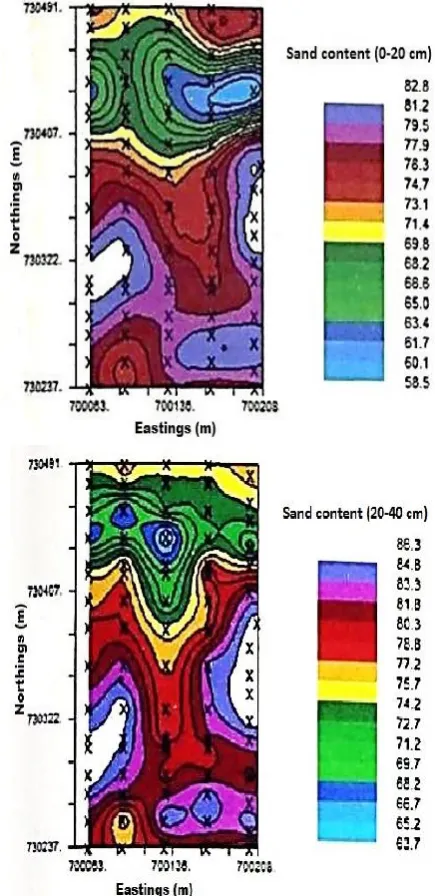
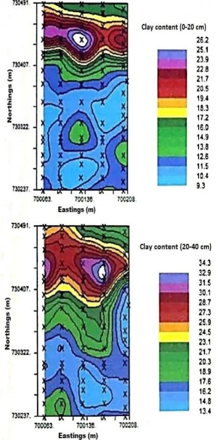
The spatial maps for particle size distribution (Figures 4a-c) showed that the entire study area was characterized by moderate to high levels of sand content, with only few patches rich in clay content. From a detailed observation of the spatial maps for sand content (Figure 4a), the parameter was found to increase from the north to south in both layers, but decreased with increasing depth along the profile. The south-western, mid-eastern and south-eastern zones in the field were observed as the areas with higher sand content in both layers. On the contrary, significant differences were not observed in silt content in both layers (Figure 4c). The main reason accountable for the poor prediction of silt content in the subsurface layer was the fact it was best-fitted by linear model, which is characterized by a pure nugget effect. The distribution maps for clay content also revealed that the parameter decreased from the north to south, with a fairly uniform distribution from east to west in both layers, except for some few patches (Figure 4b). From the spatial maps, clay content was generally less than 22 and 30% in the surface and subsurface layers, respectively. Thus, clay content was generally higher in the subsurface layer than in the surface layer.

Although the spatial variability of sand and clay contents appeared to be more continuous in the field as depicted by the natural behaviour of the best-fitted semivariogram model, the distribution of areas with higher sand content seemed to be more towards the south-western and mid-eastern zones in both layers in the field. However, very few clay patches appeared around the mid-western zone in the field. Moreover, areas with lower clay contents were found to be well distributed throughout the field. It was, therefore, assumed that these locations with lower clay contents resulted from the effects of erosion and lessivage.

[image:9.595.323.541.116.565.2]

(10)

[image:10.595.66.545.46.550.2]

Figure 1b: Kriged map for clay content (%) in both surface and subsurface layers

[image:10.595.53.270.103.545.2]

(11)

[image:11.595.31.578.118.380.2]

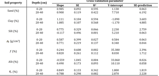
Table 3: Prediction indices for the soil properties

Soil property Depth (cm) Cross-validation parameter

Slope SE R2 _Y-intercept _{SE-prediction} Sand (%) _20-400-20 0.985 _0.900 0.092 _0.119 0.595 _0.422 1.130 _7.710 0.063 _6.192

Clay (%) _20-400-20 1.111 _1.085 0.104 _0.107 0.594 _0.568 -1.090 _-1.170 3.603 _4.885

Silt (%) _20-400-20 _-0.1170.775 0.329 _0.496 0.066 _0.001 2.230 _5.210 2.759 _0.063

(g/cm3₎ 0-20 0.587 0.399 0.027 0.584 0.063

20-40 0.771 0.219 0.137 0.340 0.044

(%) 0-20 0.244 0.608 0.002 35.380 2.396

20-40 0.820 0.261 0.112 8.030 1.712

ASt (%) _20-400-20 -0.559 _0.490 1.045 _0.173 0.004 _0.093 33.060 _10.110 8.026 _0.058

(%) 0-20 0.849 0.133 0.342 1.800 1.819

20-40 0.788 0.298 0.082 2.870 2.228

(12)

3.3.2. Spatial distribution maps and

cross-validation of soil structure indicators

From the Kriged maps, the southern and north-eastern parts of the field had bulk densities in the order of 1.50 – 1.52 g/cm3_{in the subsurface layer, however, lower values (1.38 –}

1.43 g/cm3_{) were observed in the surface layer (Figure 5a).}

The high bulk density values in the surface layer were observed in the south-eastern, with few patches in the middle part of the field as shown in the spatial distribution map. This was a clear evidence of compaction in the subsurface layer in the southern part of the field, which could have probably resulted from the accumulation of clay (i.e. clay pan), and plough pan. A general trend of increasing bulk density with depth was observed throughout the field.

[image:12.595.324.543.281.712.2]

Figure 5a: Kriged map for bulk density in both surface and subsurface layers

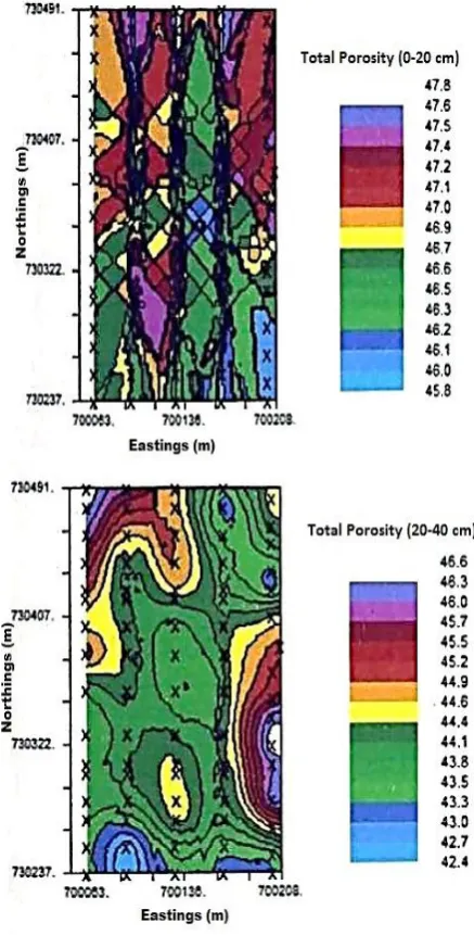
Patterns of the distribution of total porosity in both layers are presented in Figure 5b. The parameter values ranged

from 45.8 – 47.8% in the surface layer and 42.4 – 46.6% in the subsurface layer. The distribution of the property in the surface layer had no distinct trend (patchy), with higher values concentrated in the northern, mid-north-eastern and mid-south-western areas of the field as evidenced by the spatial map. The distribution of porosity in the subsurface layer, however, showed a smooth and continuous trend. The dominant parameter values (43.3 – 44.4%) were found in the middle part of the field, and stretched from the north to the south. The lower parameter values (42.4 – 43.3%) were found to be concentrated in the southern part of the field, with a few patches in the north-eastern part, while the higher values (45.7 – 56.6%) were found in the south-eastern and north-western parts of the field.

Figure 5b: Kriged map for total porosity in both surface and subsurface layers

[image:12.595.52.282.282.726.2]

(13)

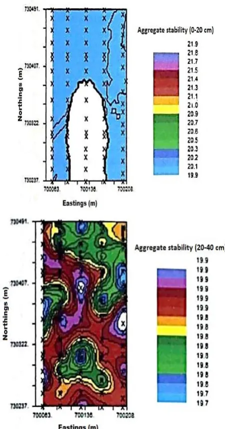
effect. Figure 5c presents the spatial map displaying the distribution of aggregate stability in the field. The distribution of the property in the surface layer ranged from 19.9 – 21.9%, with the mid-southern region stretching to the northern part of the field possessing the higher values. These zones formed approximately 8% of the total area, which implied that the remaining 92% of the field was covered by aggregates with very low stability. Based on these values, it was appropriate to conclude that aggregate stability in the entire field was low. The distribution of aggregate stability in the subsurface layer, however, showed a different trend from that in the surface layer, since the property appeared to be distributed in a patchy pattern. The best-fit semivariogram model for the property in the surface layer being linear was the main reason for its poor prediction.

3.3.3. Spatial distribution maps and

cross-validation of moisture content

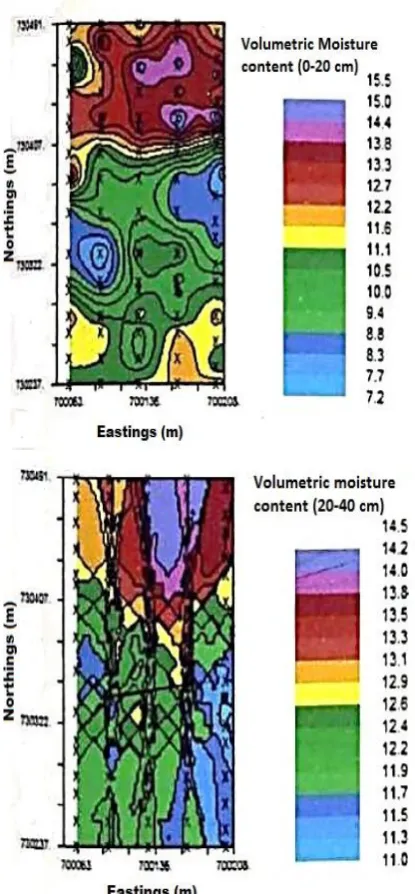
Spatial maps and cross-validation graphs prepared for volumetric moisture content through ordinary Kriging for both surface and subsurface layers are presented in Figures 6. From the spatial maps, it is evident that moisture content was maximum in both the surface and subsurface layers at the mid north-western part of the field where the clay content was highest. Cross-validation analysis showed that, the prediction of moisture content in the field was better for the surface than subsurface layer.

4. CONCLUSIONS

The presented discussions have demonstrated that soil physical properties varied in space and exhibited random spatial patterns. The distribution maps generated in the study suggest that the field could be prone to erosion since it is characterized by low aggregate stability, high bulk density, and subsequently, low porosity. The documentation of these physical properties in field scale distribution maps will allow derivation of zones of defined physical and mechanical sensitivity. This can help define management zones, which can be combined with less-dense soil samples to provide a more accurate prediction of spatial variability of soil properties for site-specific soil management under agricultural and forest land use systems.

[image:13.595.319.545.100.530.2]

(14)

[image:14.595.61.269.100.548.2]

Figure 6: Kriged map for volumetric moisture content in both surface and subsurface layers

ACKNOWLEDGEMENT

The authors wish to thank Rev. Fr. Prof. Mensah Bonsu of the Department of Crop and Soil Sciences, Kwame Nkrumah University of Science and Technology, Kumasi, Ghana for providing all the necessary support and guidance.

REFERENCES

1) J., Iqbal, J. A., Thomasson, J. N., Jenkins, P. R., Owen and F. D., Whisler (2005). Spatial variability analysis of soil physical properties of alluvial soils. Soil Science Society of America Journal, 69: 1338-1350.

2) R., Berndtsson and A., Bahri (1996). Soil water, soil chemical and crop variations in a clay soil. Hydrological Science Journal, 41(2): 171-178.

3) A. A., Jafarzadeh, H., Foroughifar, H., Torabi, N., Aliasgharzad and N., Toomanian (2010). Spatial variability of some physical and chemical properties of soil surface in Dasht-e-Tabriz Different Landforms. Geophysical Research Abstract, 12: EGU2010-336-1. 4) H. O., Tuffour, M., Bonsu, A. A., Khalid, T., Adjei-Gyapong

and W. K., Atakora (2013). Evaluation of spatial variability of soil organic carbon and pH in an uprooted oil palm field. Indian Journal of Applied Agricultural Research, 1(1): 69-86.

5) FAO/UNESCO (1990). Soil Map of the world. Revised Legend. FAO, Rome, Italy.

6) Soil Survey Staff (1998). Keys to Soil Taxonomy. Natural Resources Conservation Service, USDA, 8th ed. Government Printing Office, Washington, DC. 326. 7) P. A., Burrough and R. A., McDonnell (1998). Principles

of Geographical Information Systems. Oxford University Press Inc., New York.

8) H. O., Tuffour (2012). Spatial variability of physical, hydraulic and hydrologic properties of a tropical soil. MSc, Department of Crop and Soil Sciences, Kwame Nkrumah University of Science and Technology, Kumasi, Ghana.

9) American Society for Testing Materials. (1985). Standard test method for particle size analysis of soils. D422-63(1972). 1985 Annual Book of ASTM Standards. American Society for Testing and Materials, Philadelphia, 04.08: pp. 117-127.

10)USDA-NRSCS (2008). Soil quality indicators: Available water capacity. Soil quality information sheet, June, 2008.

11)G. R., Blake and K. H., Hartge (1986). Bulk density. In: Methods of Soil Analysis, Part 1, Physical and Mineralogical Methods, 2nd ed (Ed. A. Klute), American Society of Agronomy, Soil Science Society of America. Madison, Wisconsin, pp. 363-375.

12)W. D., Kemper and R. C., Rosenau (1986). Aggregate stability and size distribution. In: Methods of Soil Analysis, Part 1, Physical and Mineralogical Methods, 2nd ed (Ed. A. Klute), American Society of Agronomy, Soil Science Society of America. Madison, Wisconsin, pp. 425-442.

13)L. P., Wilding (1985). Spatial variability: Its documentation, accommodation and implication to soil surveys. In: Soil Spatial Variability, (Ed D. R. Nielsen and J. Bouma) Pudoc. Wageningen, The Netherlands. pp. 166-194.

14)R. B., D’Agostino (1986). Test for the normal distribution. 367-419. In: D’Agostino, R.B. and Stephens, M.A. (Eds.) Goodness-of-fit techniques. New York: Marcel Dekker.

(15)

analysis of soil fertility parameters. Precision Agriculture, 1: 5-14.

17)P., Santra, U. K., Chopra and D., Chakraborty (2008). Spatial variability of soil properties and its application in predicting surface map of hydraulic parameters in an agricultural farm. Current Science, 95(7): 937-945. 18)E. L., Aksakal and T., Öztaş (2010). Changes in

distribution patterns of soil penetration resistance within a silage-corn field following the use of heavy harvesting equipment. Turkish Journal of Agriculture and Forestry, 34: 173-179.

19)S. G., Reynolds (1970). The gravimetric method of soil moisture determination, I: A study of equipment and methodological problems. Hydrology, 11: 258-273. 20)E., Mapfumo, D. S., Chanasky and C. L. A., Chaikowsky

(2006). Stochastic simulation of soil water status on reclaimed land in northern Alberta. Journal of Spatial Hydrology, 6(1): 34-44.

21)A. W., Western, S., Zhou, R. B., Grayson, T. A., McMahon, G., Blöschl, and D. J., Wilson (2004). Spatial correlation of soil moisture in small catchments and its relationship to dominant spatial hydrological processes. Journal of Hydrology, 286: 113-134. 22)S. K., Balasundram, O. H., Ahmed, M. H., Harun, M. H. A.,

Husni and M. C., Law (2009). Spatial variability of soil organic carbon in palm oil. International Journal of Soil Science, 4(4): 93-103.

23)P., Goovaerts (1997). Geostatistics from natural resource evaluation. Oxford University Press, New York.

24)T., Tsegaye and R. L., Hill (1998). Intensive tillage effects on spatial variability of soil physical properties. Soil Science, 163: 143-154.

25)L., Cruz-Rodriguez (2004). Soil organic carbon and nitrogen distribution in a tropical watershed. MSc. Thesis. University of Puerto Rico, Mayagüez campus. 26)S., Brouder, B., Hofmann and H. F. J., Reetz (2001).