Working Paper
Modeling and Measuring Scale Attraction Effects: An
Application to Charitable Donations
Kee Yuen Lee
Hong Kong Polytechnic UniversityFred M. Feinberg
Stephen M. Ross School of BusinessUniversity of Michigan
Ross School of Business Working Paper
Working Paper No. 1380
July 2017
This paper can be downloaded without charge from the Social Sciences Research Network Electronic Paper Collection:
Modeling and Measuring Scale Attraction Effects:
An Application to Charitable Donations
Kee Yeun Lee and Fred M. Feinberg*
_______________
Kee Yeun Lee ([email protected]) is Assistant Professor of Marketing, Hong Kong Polytechnic
University, and Fred M. Feinberg ([email protected]) is Joseph Handleman Professor of Marketing, Ross
School of Business, and Professor of Statistics, University of Michigan. The authors would like to thank Jihoon Cho, Arnaud De Bruyn, Pierre Desmet, Rich Gonzalez, and Mike Palazzolo for helpful comments, as well as the Michael R. and Mary Kay Hallman Fellowship and the Asian Centre for Branding & Marketing at Hong Kong Polytechnic University for their support. This article is based on the first
author’s dissertation. Under review at Journal of Marketing Research. All comments welcome; please do
1
Modeling and Measuring Scale Attraction Effects:
An Application to Charitable Donations
Abstract
Charities seeking donations typically employ an “appeals scale,” a roster of suggested
amounts presented to potential donors, along with an “Other” category. Yet little is known about
how the amounts comprising appeals scales affect whether a donation is made and, if so, jointly
exert “pull” on its magnitude. Availing of multi-year panel data and a field experiment, we
develop a model accounting for individual level donation incidence, amount, and appeals scale
attraction effects. The model incorporates heterogeneity across donors in both upward and
downward scale point attraction, as well as in donation patterns (e.g., seasonality), and
accommodates multiple operationalizations of internal and external referents to summarize the
effects of prior donation history and scale points, respectively.
Overall results suggest that scale points do exert substantial attraction effects; that these
vary markedly across donors; that they are in fact referent-based effects; that donors are more
easily persuaded to give less than more; and that, while all scale points exert pull, influence
wanes with distance. The modeling framework applies not only in donation contexts, but
whenever an ordered categorical scale is used to collect data regarding an underlying latent
Introduction
Charities are, collectively, among the largest global financial entities. The National
Center for Charitable Statistics lists over a millionpublic charitable organizations in the United
States alone, with $1.65 trillion in collective revenue, more than Wal-Mart, ExxonMobil,
Berkshire Hathaway, and Apple combined, fully 5.3% of GDP.1 Solicitations for donations have
become a part of everyday life, with requests being made at stores, workplaces, through the mail,
various traditional media, and increasingly online (e.g., e-mail, websites, social networks).
Private citizens have been generous to charities, with over 95% of US households donating per
annum in one form or another. To help guide potential donors to both decide to give, and to give
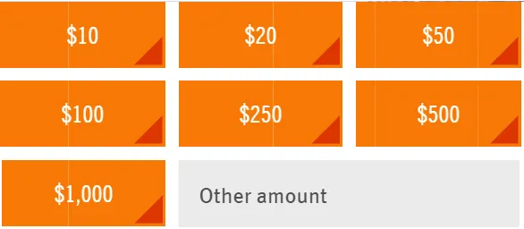
generously, charities commonly present them with an “appeals scale”; Figure 1 presents three
such scales, used for recent funding drives by the United Way (the largest US charity, with over
$3B in annual donations), Wikipedia, and the UN Foundation. Each features the most common
sort of appeals scale: a series of specific donation amounts, along with “Other” (i.e., an option to
donate whatever amount one wishes). Donors can thereby choose to give some amount not listed
on the scale, including amounts outside the range of listed values, or not at all.
Because donors can – and do, as detailed later empirically – avail of an Other amount of
their own choosing, one might question why “rational” donors would comply, choosing one of
the pre-established scale points instead of some other amount. Regardless, the mere presence of a
scale might “pull” donors upwards or downwards (hopefully the former) from what they might
have donated otherwise. Such questions are of practical concern for charities, who wish to
enhance donation drive effectiveness, and so need to assess appeals scale effects accurately.
Despite their ubiquity in charitable requests and fundraising, there is a lack of
model-
based guidance as to how appeals scales affect individual donor behavior. Part of the problem in
providing such guidance is the need for household-level, longitudinal data on both charitable
requests and outcomes – “whether” and “how much” – which charities typically possess, along
with a (suitably heterogeneous) statistical model for scale attraction effects, which they typically
do not. Here, we formulate and estimate such a model, one that incorporates heterogeneity in
individual-level “scale attraction” effects, seasonal variation in giving, and an interrelated
account for whether and how much to give, calibrated on the results of a field experiment and
donation history panel data from a French charity.
The remainder of the paper is organized as follows. We first provide a concise overview
of prior literature on scale attraction, donation behavior, reference effects, and related areas. We
then describe our empirical application, develop the model, and present both empirical results
and model comparisons, followed by general conclusions and potential for additional research.
Literature Review
The contextual effects of scale presentation on responses have been intensively examined
in social psychology over the past two decades. Schwarz’s (1999) comprehensive review
suggests that features of research instruments – question wording, format, and scaling, among
others – can substantially affect respondents’ self-reported behaviors and attitudes, echoing
earlier findings summarized by Podsakoff and Organ (1986). In particular, response scales often
act as far more than a simple “measurement device,” serving as reference frames that influence
responses (Schwarz et al. 1991).
It has long been observed that manipulating information on prior donations from others
can strongly affect donation behavior (Reingen 1982), as Shang et al. (2008) and Shang and
the role of request size on donation behavior (amount and compliance) in laboratory and field
data (Doob and McLaughlin 1989, Fraser et al. 1988, Schibrowsky and Peltier 1995, Weyant and
Smith 1987). Although contexts and methods vary across them, these studies largely confirm
scale manipulation effects, yet differ as to whether they affect donation likelihood, donation
amount, or both. De Bruyn and Prokopec (2013), in reviewing this literature, emphasize both the
lack of convergence in empirical studies of donation incidence and frequency (e.g., p. 500), and
also the importance of individual-level summaries of prior donation behavior, noting that a
“...few studies have acknowledged differences in internal reference points... but they have only
done so on the segment level.” In marketing specifically, such reference effects are a cornerstone
and have been supported empirically in dozens of studies (Kalyanaram and Winer 1995 and
Mazumdar, Raj, and Sinha 2005 provide extensive reviews for reference pricing, specifically).
We make especial use of one of the key findings from this literature: that two distinct
kinds of referents – internal and external – play a role in choice decisions. In donation contexts,
as discussed extensively by De Bruyn and Prokopec (2013), the former can be characterized by
what the donor “intends” to give, the latter by what the donor is asked to. Specifically, the
internal referent is an unobservable that must be inferred from other information (e.g., past
donation behavior), while external referents are presented at the time of the request via the
appeals scale. Both types of referent were extensively tested and verified by Mayhew and Winer
(1992) in the context of frequently-purchased consumer goods, and modeled, using an
asymmetric response function concordant with Prospect Theory, by Hardie, Johnson, and Fader
(1993), whose formulation we discuss later.
By contrast, perhaps owing to the lack of individual-specific histories, prior accounts of
and Smith (1987) found no significant difference in the average donation amount between the
“smaller request” and “larger request” conditions, only in donation rate. Yet Doob and
McLaughlin (1989) suggested, that when the “larger request” is beyond what donors can accept
(e.g., outside a latitude of acceptance; Kalyanaram and Little 1994), it exerts negligible effect:
when lower amounts were substituted in the “larger request” condition, there was a significant
difference in the average donation amount, but none in rate. Two points are relevant here: first,
this one change in referent reversed the pattern of substantive results; and, second, researchers
should consider, or model, the picture painted jointly by donation incidence and amount.
Another potential source of inconsistencies involves parametric heterogeneity. Most
previous studies could avail only of aggregate data (e.g., control / experimental group, or
segment level; e.g., Desmet and Feinberg 2003) to assess the mean scale manipulation effect
across conditions, potentially diluting the estimated effect of scale manipulation. In this regard,
De Bruyn and Prokopec (2013) were exceptional in having obtained each donor’s prior donation
before the field experiment, using it a proxy for the donor’s internal referent. Despite this
advance, the one-shot, before/after nature of their data precludes incorporating both dynamics
and “unobserved” parametric heterogeneity, which likewise plagues all prior studies relying on
cross-sectional data. By contrast, a panel of individual donors provides a superior and dynamic
platform to detect and measure scale effects. Panel data further enables us to build up an account
of individual donors’ internal referents over time, as well as provide a fully heterogeneous
account of scale attraction effects.
Lastly, no published study employing scale manipulation has provided a unified account
of both donation incidence and donation amount. Presuming whether to donate and how much to
2013). An especially appealing framework is a Type II Tobit model, which comprises accounts
of both incidence and a conditional output of interest (e.g., amount donated). Type II Tobit
models have been deployed to analyze disparate contingent consumer decisions (e.g., Ying et al.
2006 for recommendation provision and positivity, Ascarza and Hardie 2013 for usage and
retention, Shi and Zhang 2014 for store visit and spending, etc.), with the connection between
incidence and amount measured by a correlation parameter. Although not involving scale
manipulation specifically, Donkers et al. (2006) and Van Diepen et al. (2009) used such a model
in donation contexts, but with somewhat conflicting results regarding correlation; we return to
this point later when discussing our own results. In the Conclusion, we discuss a number of
behavioral theories that could in principle be assessed using the proposed model coupled with
appropriate experimental data; given the nature of our field experiment, we do not engage in
such testing here, but do indicate when our findings are consistent with prior frameworks.
Data description
Our data were provided by a French charity that conducted a large-scale field experiment
as part of a national fundraising campaign. The charity holds three fund-raising drives a year, at
Easter, June, and Christmas. Data were collected for 10 periods in total, and consist of
household-level records for the appeals scale presented to donors, whether a donation was made
and, if so, the donation amount. Donation appeals were made by door-to-door canvassing (and so
results pertain to this relatively high involvement method) to “regular” donors, who had always
been approached that way in the past; subjects were partitioned into two groups (“levels” 1 and 2)
according to their average donation amounts over the two years prior to the start of the
FF and 200 FF–399 FF, respectively.2
The charity sought to better understand the role of appeals scales in donation behavior, so
manipulated it in an experiment using random assignment. Throughout, scales (see Table 1) all
consisted of five suggested amounts, as well as an “Other” category, which allowed donors to
give what they wished. The same scale (90, 150, 250, 500, 1000 FF) was used for all subjects for
the first 8 periods of the data, and thereby helps establish a baseline. The scale was then altered
for all subjects in period 9, then again for half in period 10, where different “test scales” were
used in groups 1 (lower level) and 2 (higher).
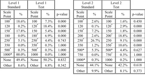
[TABLE 1 ABOUT HERE]
The charity thereby implemented a 2 × 2 design: (prior donation) “level 1” or “level 2” ×
random assignment to either a “standard” or “test” appeals scale in period 10.3 It is important to
note that the charity was collecting real donations, and therefore did not have the luxury of
‘optimally’ designing scales for experimental purposes, such as orthogonalizing (e.g., some
donors asked for less than they were accustomed to), including extreme values, and the like.
Thus, the points comprising the “test” scale for the level 2 (higher prior) donation group were,
quite sensibly for a field test, higher than those for the level 1 group, and potentially constitute a
source of endogeneity. We will explore this possibility in the sequel, by estimating the model
separately on each group and comparing individual inferences via a multivariate Cramer test.
Four hundred households in each of the four “cells” were randomly selected for analysis.
Table 2 presents descriptive statistics for each, average donation amount (per household and per
occasion), and yield rate. Level 1 and 2 differ substantially in per-household and in per-occasion
2 The charity judges regularity based on donor frequency (number of donations in past two years) and recency (periods since last donation). The distinction was applied both prior to and throughout the data window. Currency is French Francs (FF), trading during the collection window at approximately 7 to the US dollar.
3 The scale was changed twice (periods 9 and 10) for those in each of the test groups (Level 1 and Level 2), which
average donation amounts (p < .0001); this is unsurprising, as the baseline donation amount was
used by the charity to partition donors into different levels. However, yield rates are remarkably
similar across the four groups, with all between 63% and 69% (differences all ns). Moreover,
average observed donation fails to differ across the standard and test scales, within a donation
level (1: 144.7 standard vs. 148.8 test, p > .2; or 2: 268.6 standard vs. 275.4 test, p > .5). One
might conclude that there were no effects attributable to the use of the test scale. As the
forthcoming analysis will show, such a conclusion based on aggregate metrics is not only
premature, but highly misleading.
[TABLES 2 AND 3 ABOUT HERE]
Table 3 suggests a clear (aggregate) seasonal pattern in both yield rate and average
donation amount: people give more, and more often, at Easter than during June or Christmas.
The difference in yield rates is striking – nearly ¾ of respondents donate at Easter (an important
holiday in France), while just under ¼ do at the other times of year – and these proportions are
nearly identical in the level 1 and 2 donation groups (the latter, by construction, has higher
donation amounts across the board). Holding aside any aggregate patterns, there is nonetheless
sizable variation in household-level donation profiles, with many households showing a strong
preference for giving at particular times of year; this will manifest in the forthcoming model as
substantial heterogeneity in seasonality.
“Model-Free” Evidence of Appeals Scale Effects
Before building a model, one should ascertain whether there is a phenomenon worth
modeling. Table 4 presents “model-free” evidence that quantities manifest unusually strongly
when they appear on the scale, vs. when they do not; specifically, all points appearing on either
[TABLE 4 ABOUT HERE]
For Level 1, the clearest evidence for scale attraction effects can be seen when the
‘unusual’ amount of 120FF is substituted for 100FF: whereas only 0.2% of respondents donated
120FF when it did not appear on the (Standard) scale, 18.4% did when it was among the five
suggested amounts (p < 0.001 by Fisher’s exact test); a similar difference (0% vs. 6.9%; p <
0.001) is apparent for the 180FF quantity. Both of these are sensible test values, given the
~140FF average donation for the Level 1 group (see Table 2). For Level 2 donors, where the
average is ~270FF, we might expect similar effects for larger values slotted into the Test scale.
And this is precisely what we find: at 200FF (2.6% Standard vs. 18.8% Test; p < 0.001) and
350FF (1.2% Standard vs. 10.6% Test; p < 0.001). Something analogous happens when a value
is removed from the Standard scale, for example 150FF in either Level 1 (17.8% Standard vs. 5.4%
Test; p < 0.001) or Level 2 (7.2% Standard vs. 1.8% Test; p < 0.001). 4 By contrast for all values
included on both scales, as well as choosing not to give – that is, “None”, 250FF, 500FF in Level
1, and “None”, 500FF in Level 2 – pairwise differences are all ns (p > .5 in all five cases).
Thus, it seems fair to conclude that the appeals scale points succeed in “relocating” mass
in the PDF for donation amounts. But this fails to answer several critical questions: Are all
donors equally susceptible to scale effects?; Do all points ‘pull’ equally well?; Is the pull
stronger upwards or downwards?; What is the role of prior donation history?; Are these truly
reference effects?; among others. To answer these basic questions requires that one go beyond
summary “model free” metrics and fashion a model calibrated on the individual histories of
many households. Although we are not the first to examine appeals scales in individual
donations (e.g., De Bruyn and Prokopec 2013), the model is indeed the first, to our knowledge,
that attempts to quantify appeals scale attraction effects. The presentation will therefore be
suitably general, although the discussion will largely be tailored to our specific context of
charitable donations.
Model Development
Internal and External Referents
The model hinges on two constructs, as discussed previously and at length in the review
of the literature by Mazumdar, Raj, and Sinha (2005): that, for a particular donor, each request
can be associated with both an internal referent ( ), which the analyst can relate to prior
donation history, and external scale-point-based referents ( ); if an appeals scale contains
multiple points, we denote the kth as , .
A key modeling task is appropriately summarizing the effects of both the internal (IR)
and external (ER) referents. Both admit different operationalizations, which can be empirically
tested for a given model via standard fit metrics. Prior literature offers several options for IR,
including most recent prior value (e.g., Krishnamurthi et al. 1992) and variously weighted
amalgams of past realizations (e.g., the summary in Table 1 of Briesch et al. (1997). We test five
such specifications, two specifically tailored to account for seasonal donation variations: the
average of all prior observed donation amounts (IR-1); the last observed donation amount (IR-2);
the average observed donation amount at the same time of year (IR-3); and the last observed
donation amount at the same time of year (IR-4), and a geometrically-smoothed version (IR-5)
that estimates the relative weight (α) on the last observed value (i.e., equation 3 of Mazumdar et
al. 2005). Note that IR-2 is a special case of IR-5, with α = 1. These should be viewed not as
mental constructs, which is in any case unverifiable, but as univariate autoregressive summary
That the external reference (ER) points are observable might make them appear simple,
or simpler, to account for. This might be so were there only a single requested amount. But, in
practice, there are several, and so it is unclear how they exert their “joint pull”: perhaps the
extremes are differentially noticed, or discounted; or only those nearest the internal referent have
any influence; or some summary measure of all points (like the average or median); or
something else entirely.5 De Bruyn and Prokopec (2013) speak directly to such weighting
schemes, finding “leftmost anchor” exerted the strongest pull; this echoed a prediction of
Schibrowsky and Peltier (1995), but is contrary to, for example, extremeness aversion (Simonson
and Tversky 1992). We therefore consider a wide range of possibilities in the absence of prior
theory to suggest how a group of referents exert collective influence, an intriguing open issue
that our data and model may help address. Specifically, we test whether influence is exerted by:
all scale points (ER-1); the two points closest the internal referent (ER-2); the largest and the
smallest points (ER-3); the median (i.e., middle) point (ER-4); the mean of all points (ER-5); and
all scale points with various weighting schemes, equally (e.g., with relative weights 1-1-1-1-1;
6); in a V-shape (3-2-1-2-3; 7); inverse-V (1-2-3-2-1; 8); increasing (1-2-3-4-5;
ER-9); and decreasing (5-4-3-2-1; ER-10).
Modeling Scale Attraction Effects
If the appeals scale “pulls” donors’ internal referents towards the presented external ones,
these separate pulls can cumulate in their effects. A simple metric for scale point influence is its
“compliance degree,” which we describe next.
1. Compliance Degree
We define , “compliance degree” of the kth external reference point as the
proportional increase (or decrease) from a donor’s internal reference point ( ) to an external
one ( , ). Specifically (with DA = Donation Amount received):
/ , (1)
For example, if a donor has (latent) internal referent $100, but is asked for $300 and partly
complies by giving $150, = ($150 - $100) / ($300 - $100) = 25%. That is, the donor
“came up 25%” from a $100 baseline. It is convenient to define the distance, , between the kth
external and the internal referent as a (positive) ratio:
‖ , ‖/ (2)
This allows both compliance degree and pulling amount (described later) to be expressed as
dimensionless quantities, which in turn helps to unify the model; for example, comparing a donor
planning to give $10, but gave $20, to one planning to donate $100, but asked for $200.
We model both upward and downward “compliance degree curves”, which satisfy three
properties: (1) 1 for 0: “Maximal compliance occurs near donors’ internal
referents”; (2) decreases monotonically in : “Compliance is worse for requests further
from the internal referent”; and (3) 0: “Compliance can’t be worse than zero.” Properties
1 and 2 suggest donation is highly responsive to asking for amounts close to what was ‘planned’
(the internal referent), but increasingly less so for distant amounts. Property 3 simply suggests
that requests can be ignored, but do not literally repel donors from a scale point.
Among the many ways to specify compliance degree curves satisfying these three
properties, we select a translated gamma kernel function, for two reasons. First, it provides a
identified, given the small number of responses per donor during the data window. Second, the
gamma kernel enables the pulling amount curves (described later) to follow a non-multimodal,
yet flexibly-shaped, distribution. Specifically:
/ ; exp , ,
exp , , (3)
where 0 is the gamma kernel scale parameter; shape parameter is set at 1.6 When , , we have an “upward” compliance degree curve, and otherwise a “downward” one. Since the
scale parameter ( ) must be positive, we specify or , where and are the “upward” and “downward” parameters in (3). Note that = does not imply identical
upward and downward curves, because the domain of the downward curve is bounded by 100%,
since one cannot give less than zero (i.e., a 100% decrement).
Although our model is novel in its account of scale attraction effects, specifically, it is
hardly the first to accommodate asymmetric (i.e., upward and downward) reference effects in an
empirical context. Hardie, Johnson, and Fader (1993) built a model that explicitly encoded the
possibility of different weighting of both price and quality deviations (from one’s last purchase)
in utility, estimating the model on packaged goods. Our formulation, while similar in some
respects, further accounts for the role of multiple external referents (the appeals scale), a variety
of internal referent specifications, nonlinearity in utility, latent correlation in incidence and
amount, and a more flexible (hierarchical Bayesian) account of “unobserved” heterogeneity.
2. Pulling Amount
The pulling amount is the size of effect exerted by a scale point, the product of
compliance degree and distance between the internal ( ) and the kth external referent ( , ):
|| , || (4)
Pulling amount captures a trade-off between asking for too little and too much: If a charity asks
for just a bit more than the internal referent, compliance ( ) may be high, but the potential
surplus (|| , ||) is small. Conversely, asking for too much leads to low compliance and
large surplus. This trade-off (where the extremes are literally zero) guards against ‘highly
influential’ scale points being placed too close or too far from internal referents.
Equation (4) implies that both “upward” and “downward” pulling curves also follow a
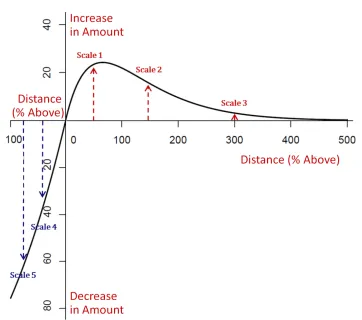
gamma kernel, with shape parameter 2 and scale parameters exp and exp . As depicted in Figure 2, these curves can take a variety of shapes: the upward pulling curve has domain
0, ∞ , is unimodal (and thus has a unique maximum), with zero at the origin and asymptoting to zero for large d (for any . The domain of the downward pulling amount curve is [0,1]; it is
unimodal (with unique maximum) if 0, and is monotonically increasing otherwise (with maximum at 1). These internal maxima map bijectively to { , }, and so provide an
equivalent projection of the parameters onto a meaningful metric: which upward and downward
scale amounts (proportions above the internal referent) provide the strongest expected deviations.
Appendix C derives closed-form expressions for these, which we will use for graphical purposes.
[FIGURES 2 AND 3 ABOUT HERE]
3. Accumulating Scale Attraction Effects
Because real appeals scales invariably comprise multiple points, their effects need to be
somehow combined. Figure 3 illustrates the “accumulated pulling amount” accruing from
two lesser – are depicted, with upward and downward curves on either side of the graph.
Because the charity did not change scales many times across the 10 periods (nor within
each of the four donation groups), identifying interactions among scale points is not possible.
Thus, the effect of each scale point is modeled separately. This is partly mitigated by the
weighted-averaging schemes explored for the “accumulated pulling amount”, or APA. In general:
∑ ; 1, ,
1, , (5)
Summing the scale pulls (i.e., 1) is simple and intuitive, but has a shortcoming in the effect of including additional scale points (not testable here, as the charity fixed this at 5). For
example, given internal referent 50, the APA of the four-point scale {9, 11, 99, 101} would be
about twice as strong for the two-point scale {10, 100}, which seems unrealistic. Averaging
( 1/k) addresses this, but raises other problems. For example, if a donor is asked for $2000 when the planned amount is $100, the real effect of such a “distant ask” might be negligible.
However, equal weighting suggests a sizable effect, which again seems unrealistic. A simple
rescaling, i.e., ∑ , addresses both issues, while retaining proportionality. As
mentioned previously, data limitations (indeed, for any data likely to be available in a
charity-based study) precluded measuring , leading to empirically testing the 10 weighting schemes
of ER-1 through ER-10.
General Model (Type II Tobit)
We outline the general model structure, which affords a “dimensionless” account of pulling
effects, so that heterogeneity can be specified across the log-scale for donation amount. As
∗ (6)
∗ , where:
1, if ∗ 0; 0 otherwise
∗, if 1; unobserved otherwise
, ~ 0, ; 1
The subscripts i and t (for donor and time) are suppressed, and and are covariates in the
selection (s) and amount (a) equations, respectively, which we detail below.
In the amount equation, ∗ denotes the log of the latent donation amount, which is
observed only when a donation is made, that is, when = 1, which occurs when the latent
variable ∗ 0. The errors ( , ) are bivariate normal, with variance of fixed to 1 for identification. It is important to note that we model the logarithm of donation amount, for several
reasons: first, it allows to be plausibly homoscedastic; second, it allows all effects in the
amount equation to enter multiplicatively; and third, it allows for coefficient heterogeneity to act
on a dimensionless quantity, which we address in detail shortly.
The amount equation (for ∗) contains two deterministic components. The first is the
sum of a donor’s internal referent ( ) and the accumulated pulling amount (APA), which can be
positive or negative. The second is all factors ( ) that affect the donation, other than those
stemming from the appeals scale. Scale-based effects do not appear directly in the selection
equation, because in our data all scales used were set in “reasonable” ranges for every donor
(recall that these were real donors, and the charity was reluctant to alienate them with
unrealistically high requests, or lose funds with low ones). The appeals scale exercises influence
on donation incidence via the correlation, . [A model was estimated allowing for scale effects in
Explanatory variables and Heterogeneity
1. Explanatory variables Selection equation
The selection equation contains three types of explanatory variable ( ), which we detail
subsequently: seasonal indicators, (log of) prior donation, and “level” fixed effects. Table 3
reveals strong aggregate seasonal variation in donation likelihood, by far highest at Easter. Three
dummies – Easter ( ), June ( ), Christmas ( ) – represent when the request occurred. The
log of (1+ amount the donor gave on the last request), donated , is included to examine carryover effects, and is 0 when no donation takes place.7
Although Table 3 suggests only modest differences in yield rate between the “larger”
(level 2) and “smaller” (level 1) donation groups, we include a Level dummy ( ) among the
selection covariates, to allow for potential differences in baseline donation likelihood after
accounting for seasonal patterns. Coefficients for the three seasonal dummies, the log-donation
lag, and the level dummy, are denoted , , , , and , , respectively. In the experiment, donors were randomly assigned to receive either a Standard or a Test appeals scale
(during period 10), so no dummies were entered for this difference (in either selection, or
amount). Doing so failed to improve fit, in any case, so we do not discuss these again.
Amount Equation
Based on examination of the data and unimproved fit of models including them, seasonal
dummies are not included in the amount equation; the somewhat higher amounts indicated at
Easter in Table 3, for example, will be well-explained by other covariates, like lags in setting
“internal” referents (such as in IR-3 and IR-4). The data suggested great household variation in
when to give, not how much; and that household-level seasonal variation in amount (not
incidence) is small for most donors. Lastly, although donation amount is mainly predicted by a
donor’s internal referent and scale effects, a level dummy ( ) is included to account for the
difference in baseline donation amount between the two groups, denoted , .
Heterogeneity
It is critical to incorporate “unobserved” heterogeneity, which we do in several ways.
First, we model heterogeneity in the seasonal dummies for the June and Christmas coefficients
( and ).8 Importantly, since the model intends to capture scale attraction effects, the two
“pulling” parameters ( and ) in the amount equation are heterogeneous. If for example
were homogeneous, each donor is presumed equally ‘elastic’ in being cajoled upwards. Our
results will in fact strongly weigh against this presumption. To test implications across models at
the individual level, we will use a multivariate generalization of the Kolmogorov-Smirnov test,
the Cramér-von Mises statistic, on the individual-level joint posteriors for , .
Our formulation therefore specifies four heterogeneous parameters, to be recovered from
the relatively short data window of 7 occasions, roughly 3 of which resulted in donations, on
average. Although this may appear ambitious, simulations showed good recovery for all four
heterogeneous parameters, and excellent recovery of the others.
Estimation
The full model (see appendix A) is estimated using Markov chain Monte Carlo methods.
Data augmentation (Tanner and Wong 1987) essentially converts the model to a Bayesian
Hierarchical Seemingly Unrelated Regression. We obtain posterior draws via
Metropolis-within-
Gibbs algorithms: Gibbs sampling if the full conditional of a parameter block is of known form,
and Metropolis-Hastings, with a random walk proposal (Chib and Greenberg 1995), otherwise.
We set diffuse priors for all parameters of interest; detailed procedures appear in Appendix B.
All estimates are based on 100,000 draws. We discard the first 50,000 draws for burn-in, and use
the last 50,000 (thinned to every tenth) to calculate posterior densities. Trace plots and standard
diagnostics indicated convergence of all key parameters.
Results
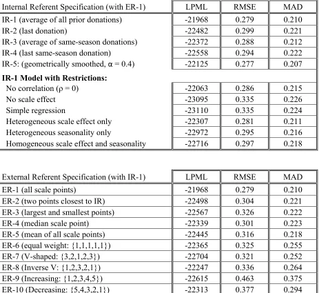
Model selection was based on LPML (log pseudo-marginal likelihood) which, as noted
by Chen et al. (2008) works particularly well for GLM-type models, and more generally by Chen
and Kim (2008). For brevity, we only present full estimation results for the model with IR-1
(average of all observed donation amounts) and ER-1 (all scale points), as these provided the
best fit compared with all possible combinations of the other internal and external references
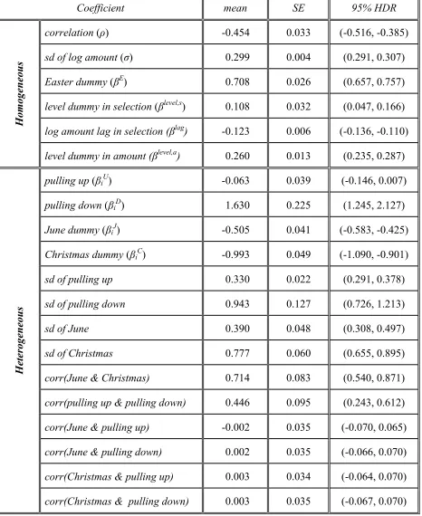
point formulations (i.e., IR 2-5 and ER 2-10). Table 5 summarizes posterior means and standard
errors for all parameters. Detailed model comparison statistics appear in Table 6.
[TABLES 5 AND 6 ABOUT HERE]
Error Correlation in Selection and Amount equations
The mean of the marginal posterior for the error correlation, ρ = -0.454, between
selection and amount is negative, and the 95% highest density region (-0.516, -0.385) is far from
zero. This suggests that unmeasured factors influencing selection are correlated with those
influencing amount, and operate in opposite directions. For example, a donor might, for some
“latent” reason, be saving up to give a larger donation, lowering frequency and raising amount;
or, conversely, may compensate for not having given for a while with a larger donation. The size
research using related model formulations; for example, Donkers et al. (2006) found the
correlation to be very slightly negative (-0.033; p < .001), while Van Diepen et al. (2009) found
it to be large and positive, with a 99% credible interval of (0.946, 0.970). Very small
correlations may fail to correct for potential selection biases, or could reflect substantial,
independent sources of error in each equation. Conversely, a large correlation might suggest
nontrivial variables omitted in both equations. It is difficult to generalize such results, since our
model accounts for scale attraction effects, while prior ones do not. We did, however, find
significant, moderate, negative values of ρ across a very wide range of candidate models, indicating that error correlation needs to be accounted for in our data.
We note in closing that ρ is a residual correlation, and is distinct from any “model-free”, observable correlation that might exist in the data, like between number and amount of donations
made. This latter sort of correlation is computed across donors, but ρ could be assessed even for a single donor, if his/her donation history were long enough. Lastly, ρ is theoretically and empirically distinct from scale attraction effects per se: for example, although not having given
in (say) the first two periods may make it more likely one will donate in the third (or donate
more in the third), it should not make it more likely that one will move closer to a scale point.
Selection: Seasonality
Comparing the Easter coefficient (0.708) to the (heterogeneous) ones for June and
Christmas (-0.505 and -0.993, respectively) accords with the observation that giving was much
more likely for Easter, on average. There is a substantial seasonal heterogeneity: the SDs of
individual-level parameters for June and Christmas are 0.390 and 0.777, respectively. The large
(0.714) correlation between these individual-level parameters largely reflects the fact that June
time; nevertheless, the concordance of the model’s parameters with aggregate benchmarks is
reassuring.
Level Dummies and Lagged Log-Amount
The level dummy is moderately significant (mean 0.108, SE 0.032) in selection, but
strongly positive in amount (mean 0.260, SE 0.013). So, as aggregate statistics suggest, level 2
donors give far more than those in level 1, but with modest difference in yield rates. The
coefficient of the log-donation lag in selection is significantly negative (mean -0.123, SE 0.006),
indicating that a larger donation amount last time leads to being less likely to give at all this time.
“Pulling Effects”: Gamma Kernel Parameters in Donation Amount
The values of and determine each donor’s degree of compliance (“pull”) to the scale points above and below the internal referent. Because the domains of the two compliance
curves differ, we should not compare directly to . Figure 4A in some sense encapsulates
our main results: the upward and downward pulling parameters (posterior means of and ) for each donor. There is clearly a good deal of heterogeneity, indicating differing degrees of
susceptibility to the appeals scale, despite only modest differences in prior donation behavior.
That is, although these donors may seem similar in terms of observed donation behavior, they
apparently are not in terms of how swayed they are by the appeals scale.
[FIGURE 4 ABOUT HERE]
By allowing a bivariate density for ( , ), the model helps assess overall scale compliance. Specifically, we find a substantial correlation (0.446) in these values, suggesting
that donors who are “upward compliant” tend to be “downward compliant” as well. There is no a
priori reason to expect these should be correlated at all, let alone positively, and we believe this
maps to the joint distribution of maximal pulling amounts (see Appendix C), those scale values
associated with the strongest overall effects; we do not call these “optimal”, since a large
downward pull is to be avoided. Heterogeneity in ( , ) leads to substantial variation in maximally effective scale values. The model suggests that the scale point with maximal upward
pull, which varies across donors, ranges from 57.2% to 245.5%, with a mean of 94.9%, above
one’s internal referent, which seems reasonable.9 This substantial variation has an important
implication: that it may be possible to substantially increase donations by personalizing an
appeals request, based on each donor’s history, although such dynamic optimization is nontrivial,
and has similarly stringent data history requirements.
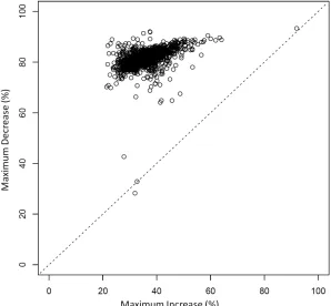
Figure 4B translates the model’s key substantive findings into the context of the original
data, specifically: How much does the maximally-effective “ask” value (either up or down) pull
from the internal referent? It depicts, across donors, this maximal percentage increase and
decrease (see appendix C for derivation), allowing a direct comparison of upward vs. downward
scale attraction “strengths”; this was not sensible using the information on ( , ) in Figure. 4A, given their different domains of operation. Maximum percentage increases range from 21.1% to
90.3% (mean = 34.9%; SD = 5.4%); decreases from 31.2% to 94.5% (mean = 82.0%; SD =
3.1%). These means suggest, unsurprisingly, that donations are more readily deflected downward
than upward. Figure 10 suggests that the maximum percentage decrease is greater than the
analogous increase for most donors: 81.6% of the donors lie above the diagonal (dotted) line.10
This is nonetheless reminiscent of the asymmetric effects in Desmet and Feinberg (2006), whose
lack of individual-level data precluded any distributions across donors, and De Bruyn and
9 Discussions with a large university’s fundraising team suggested that the success of such “upping” dropped nearly to zero when appeals hit 200% above a donor’s typical or last donation amount.
10 This hypothesis about “up” vs. “down” differences can be tested. For our 1600 participants, “down > up” for
Prokopec (2013), who only had one-shot (i.e., “before” and “after”) data unsuited to modeling
heterogeneity or carryover effects.
Model comparisons
The model and data together provide clear evidence of scale-based effects on the distribution of
donations. But one might reasonably question whether these were strongly dependent on the
particular form of the model, five of its elements in particular: 1) internal reference point
specification; 2) external reference point specification; 3) including correlation (Type II Tobit),
seasonality, and scale effects; 4) incorporating response heterogeneity; and, perhaps most
important, (5) whether the scale should operate as reference effects at all, as opposed to merely
summary covariates. We examine each of these in some detail, to assess relative “contribution”
to overall model fit, comparing the five internal referent specifications (IR-1-5) and ten external
reference formulations (ER-1-10), as described in the model development section.11 We refer to
the model with all the aforementioned components – internal and external referents; error
correlation; seasonality; heterogeneity – as the “full model”. Alternative models include those
lacking: error correlation (“no correlation”), scale effects (“no scale effect”), both (“simple
regression”), various forms of heterogeneity (i.e., homogenous seasonality, homogenous scale
effects, and both), and reference effects altogether (“no reference effects”), as explained below.
Owing to short donation histories (which preclude ‘squandering’ an entire year for
prediction purposes), we compare fit in-sample, assessed via LPML, mean absolute deviation
(MAD) and root mean square error (RMSE) for donation amount predictions; these appear in
Table 6. The proposed model (“full” with IR-1, ER-1) provides a better fit than all alternatives
via the LPML measure, and very nearly so using MAD and RMSE, surpassed only by geometric
smoothing (with an optimal smoothing carryover near 0.4); moreover, including error correlation
and scale effects improves fit regardless of internal reference formulation (IR1-5) and the
inclusion of heterogeneity.12
Table 6 also allows us to judge relative contribution to overall model fit: scale effects
easily best both correlation and seasonality. For example, failing to account for scaling effects
(“no scale effect”) inflates RMSE approximately 20% (i.e., to 0.335 from 0.279); the
corresponding figure for removing correlation alone is ~2.5%. Dropping heterogeneity entirely
entailed a ~6% RMSE decrease (to 0.297), but only ~0.7% of this was attributable to seasonality
(RMSE = 0.281). These comparisons suggest that scale attraction effects may explain more
variation in giving than those typically modeled in prior donation research combined, although
only additional applications can verify whether this holds generally.
In terms of internal reference point specification, IR-1, the average of all prior donation
amounts appeared to dominate across the board, based on LPML. The degree of dominance was
nontrivial, as high as 7.1% in RMSE; to our knowledge, such a test of ‘internal’ referents is
unprecedented in donation contexts. Given this pattern of results, we restrict our attention to the
“full” model with IR-1, and the lower portion of Table 7 summarizes fits of the ten external
reference specifications (ER 1-10) for this model. ER-1, with all five scale points included,
clearly dominates, by RMSE degrees ranging from 8% (vs. ER-4, for the median scale point) to
66% (vs. ER-9), for linearly increasing emphasis on higher scale points. We hesitate to term this
a general finding in the absence of data capable of assessing these weights (perhaps even
heterogeneously) via estimation, but the degree of advantage for ER-1 over the other nine
alternatives is at the very least suggestive, and differs from De Bruyn and Prokopec’s (2013)
finding that the lowest scale point exerts the strongest influence (e.g., ER-10: RMSE = 0.377, or
a 35% increase), although their empirical setting was somewhat different.
Regardless, the “full” model with IR-1 and ER-1 was verified to provide the best fit to
the data among the 2 × 2× 2 × 2 × 5 × 10 (scale effects?; scale effect heterogeneity?; seasonality
heterogeneity?; error correlation?; IR1-5; ER1-10) design. However, this precludes the
possibility that the scale effects were not reference effects, which we take up next.
Division into Levels 1 and 2
As reported earlier, the charity divided prior donors for the experiment in its customary
manner, based on prior donation amounts. This is entirely sensible, given the potential for loss,
and even the carefully randomized study of De Bruyn and Prokopec (2013) “...constructed a
customized appeal scale for each donor, tailored to both his/her last donation and the assigned
experimental condition”, introducing a potential for endogeneity. However, as Dorotic et al.
(2014) report in the context of Loyalty Programs (LP), “From discussions with the LP manager,
we know that only the frequency of the mailings is endogenous; its timing is not set based on
individual behavior,” and so they can “easily correct for the endogeneity”. In our study, timing
of requests is fixed and identical across groups (Levels 1 and 2; Standard and Test), and only
groupwise manipulations (i.e., for Levels 1 and 2 separately) are involved. It is possible to
simply re-estimate the model for each Level alone: while this reduces statistical power, it ensures
that the results for each individual are informed only by the scale used in that individual’s group
(which cannot be ensured in the hierarchical Bayes set-up used to analyze the Level groups
effects, ( , ), and test each of the 800 Level 1 and 800 Level 2 individual’s bivariate
posterior from the “Levels estimated separately” model to those previously obtained: none of the
1600 showed significant differences at the .05 level.
Testing against Non-Referential Scale Effects
The model-free evidence presented at the outset strongly suggests that respondents do
react to the presence of the appeals scale, even though they have the option of ignoring it and
donating whatever amount they want, or nothing at all. We assessed the importance of scaling
effects in our model by estimating a nested version with the scaling removed entirely (Table 6,
“no scaling effects”). But this raises the question of whether the hallmark of reference effects –
(potentially asymmetric) pulling up and down, relative to a referent – is actually present in our
data. The proposed model (6) is for the deviation between the donation amount and
, the internal referent adjusted for (asymmetric) pulling effects. Another possibility is to
retain summary measures of both IR and ER, but without reference effects, specifically. This
entails removing entirely, and instead including among the regressors (i.e., along with
, ) summary measures of the appeals scale points (i.e., ER-1-10), heterogeneously.13
It is possible to compare these results (for all possible configurations of IR and ER) via
LPML; in every case, the results are inferior to the proposed model (i.e., the “full” model, with
IR-1 and ER-1). For the basis of explicit comparison, we replicated all the results of Table 6 for
this revised model, and LPML ranges from -23419 (for IR-1, ER-2) to a best value of -22842
(for IR-1, ER-3), compared to the proposed model’s best value -21968 (for IR-1, ER-1). {MAD,
RMSE} were fairly stable for the “no reference effects” models, hovering near {0.298, 0.226} vs.
{0.279, 0.210} for the proposed model. That this revised “scale effects, but no reference effects”
13 We are grateful to an anonymous reviewer for pointing out this distinction, and suggesting this explicit model as a
model makes use of the same data and identical operationalizations of both IR and ER, yet fits
less well across the board – approximately 10% in log-donation, based on MAD – lends credence
to the documents pulling effects being reference effects, specifically.
Conclusion
Charities have long relied on appeals scales as cornerstones of their donation requests,
setting them based on experience and enlightened guesswork. By contrast, the model developed
here offers a heterogeneous, joint account of donation incidence and amount, while accounting
for the asymmetric effect of the appeals scale. Moreover, different specifications for internal and
external reference point theories can be assessed via model comparison.
Results suggest that variation across donors in scale attraction effects can be substantial.
Such a finding depends critically on the availability of donation histories, explaining its absence
from prior studies. A moderate, significantly negative, correlation between donation incidence
and amount indicates the potential pitfalls of providing separately accounts, echoing similar
results long-accepted in brand choice (e.g., Lattin and Bucklin 1991). In terms of internal and
external referents, we found that the mean of the previous donation amounts (internal referents)
and including all points in an appeals scale (external referents) offered the best fit with our data,
compared with a wide variety of alternatives, as suggested by prior literature (e.g., Briesch et al.
1997). The developed model can apply well beyond the domain of charitable requests, to any
situation where different interval or ordered categorical scales are used. Indeed, it may be
possible to leverage the model to not only detect, but correct for, many of the sorts of scaling
artifacts widely documents by consumer researchers (e.g., Schwartz 1991, 1999).
Field studies of this nature entail inevitable limitations. Charities are less concerned with
losses. In our study, for example, appeals scale amounts roughly tracked prior donation level in
each segment, instead of being orthogonalized or randomized. Second, lack of substantial
within-donor appeals scale variation allowed us only to test various weighting schemes, as opposed to
estimating the scale points’ relative influence, let along heterogeneously. Third, the optimal
number of points can only be ascertained if these were systematically varied. And finally,
because the appeals scales used by the study both historically and in the experiment contained
only ‘reasonable’ amounts, effects of extreme scale points, such as ignoring them or even of
alienating donors, await verification. Despite these data limitations, the model showed clear and
strong evidence for scale attraction effects, in both upward and downward directions, and that the
degree of attraction varied nontrivially across donors.
We have knowingly avoided trying to engage in tight tests of specific behavior theories
that, suitably interpreted, might make specific predictions about which scale points would be
relatively influential. A prime example is Configural Weight Theory (e.g., Birnbaum et al. 1992),
which suggests that a scale’s point’s influence depends on how it compares, typically ordinally,
with other points and external anchors. Tests of such theories, including range theory (e.g.,
Janiszewski and Lichtenstein 1999), extremeness aversion (e.g., Simonson and Tversky 1992),
etc., await tighter controls than are typically available in field data, as well as specific
mathematical formulations amenable to statistical estimation on individual-level data, although
some progress has been made on that front, e.g., for the compromise effect (Kivetz, Netzer, and
Srinivasan 2004).
Some of the data limitations suggest clear directions for future experimental and field
research. First and foremost would be some scheme for orthogonalizing appeals scale amounts
aspects of the scales themselves, like median and range, to be not merely measured in terms of
influence, but optimized. Future research might also identify subtleties of weighting: do some
respondents ignore endpoints, while others anchor on them? Experiments could similarly include
extreme scale points, to see whether they are ignored entirely, lead respondents not to donate at
all, or something more subtle. Lastly, the present data set could not address the persistence of
scale attraction effects, specifically, the degree to which they may be self-correcting, which
informs whether external anchors can effectively increase total contribution over a planning
horizon, what fundraisers refer to as “laddering”; assessing such issues rigorously would likely
require multiple independent scale manipulations in a field setting. Regardless, any such data
could be analyzed through variants of the basic framework employed here, and would help
validate cross-study norms about scale point attraction effects, as well as tentatively suggest
References
Andrews, R. L., A. Ainslie, I. S. Currim. 2008. On the recoverability of choice behaviors with
random coefficients choice models in the context of limited data and unobserved
effects. Management Science B54 (1) 83-99.
Ascarza, E., B. G. Hardie. 2013. A joint model of usage and churn in contractual settings. Marketing
Science 32 (4) 570-590.
Birnbaum, M. H., G. Coffey, B. A. Mellers, R. Weiss. 1992. Utility measurement: Configural-weight
theory and the judge's point of view. Journal of Experimental Psychology: Human Perception
and Performance 18 (2) 331-346.
Briesch, R. A., L. Krishnamurthi, T. Mazumdar, S. P. Raj. 1997. A comparative analysis of reference
price models. Journal of Consumer Research 24 (2) 202-214.
Chen, M. H., S. Kim. 2008. The Bayes factor versus other model selection criteria for the selection of constrained models, in Bayesian Evaluation of Informative Hypotheses (pp. 155-180).
Springer, New York.
Chen, M. H., L. Huang., J. G. Ibrahim., S. Kim. 2008. Bayesian variable selection and computation
for generalized linear models with conjugate priors. Bayesian analysis, 3 (3) 585.
Chib, S., E. Greenberg. 1995. Understanding the Metropolis-Hastings Algorithm. American
Statistician 49 (4) 327-335.
Croson, R., J. Shang. 2013. Limits of the Effect of Social Information on the Voluntary Provision of
Public Goods: Evidence from Field Experiments. Economic Inquiry, 51(1), 473-477.
De Bruyn, A., & Prokopec, S. (2013). Opening a donor’s wallet: The influence of appeal scales on
likelihood and magnitude of donation. Journal of Consumer Psychology, 23(4), 496-502.
Desmet, P., F. Feinberg. 2003. Ask and ye shall receive: The effect of the appeals scale on consumers’
donation behavior. Journal of Economic Psychology 24 349-376.
Donkers, B., R. Paap, J. Jonker, P. Franses. 2006. Deriving Target Selection Rules from
Endogeneously Selected Samples. Journal of Applied Econometrics 21 549–562.
Doob, A., D. McLaughlin. 1989. Request Size and Donations to a Good Cause. Journal of Applied
Social Psychology 19 (12) 1049-1056.
program when customers choose how much and when to redeem. International Journal of Research in Marketing 31 (4) 339-355.
Edwards, Y., G. Allenby. 2003. Multivariate Analysis of Multiple Response Data. Journal of
Marketing Research 40 (3) 321-334.
Fraser, C., R. Hite, P. Sauer. 1988. Increasing Contributions in Solicitation Campaigns: The Use of
Large and Small Anchor Points. Journal of Consumer Research 15 (3) 284-277.
Hardie, B. G., E. J. Johnson, P. S. Fader. 1993. Modeling loss aversion and reference dependence
effects on brand choice. Marketing Science 12 (4) 378-394.
Janiszewski, C., D. R. Lichtenstein. 1999. A range theory account of price perception. Journal of
Consumer Research 25 (4) 353-368.
Kalyanaram, G., J. Little. 1994. An Empirical Analysis of Latitude of Price Acceptance in Consumer
Package Goods. Journal of Consumer Research 21 (3) 408-418.
Kalyanaram, G., R. Winer. 1995. Empirical Generalization from Reference Price Research.
Marketing Science 14 (3) 161-169.
Krishnamurthi, L., T. Mazumdar, S. Raj. 1992. Asymmetric Response to Price in Consumer Brand
Choice and Purchase Quantity Decisions. Journal of Consumer Research 19 (3) 387-400.
Kivetz, R., O. Netzer, V. Srinivasan. 2004. Alternative models for capturing the compromise
effect. Journal of marketing research. 41 (3) 237-257.
Lattin, J., R. Bucklin. 1989. Reference Effects of Price and Promotion on Brand Choice Behavior.
Journal of Marketing Research 26 (3) 299-310.
Mayhew, G., R. Winer. 1992. An Empirical Analysis of Internal and External Reference Prices
Using Scanner Data. Journal of Consumer Research 19 (1) 62-70.
Mazumdar, T., S. P. Raj, I. Sinha. 2005. “Reference price research: Review and
propositions.” Journal of marketing 69 (4) 84-102.
Podsakoff, P. M., D. W. Organ. 1986. Self-reports in organizational research: Problems and
prospects. Journal of management, 12 (4) 531-544.
Reingen, P. 1982. Test of a List Procedure for Inducing Compliance with a Request to Donate
Money. Journal of Applied Psychology 67 (1) 110-118.
Fundraising Context. Journal of Direct Marketing 9 (1) 8-16.
Schwarz, N., H. Bless, G. Bohner, U. Harlacher, M. Kellenbenz. 1991. Response Scales as Frames of Reference: The Impact of Frequency Range on Diagnostics Judgements. Applied Cognitive
Psycology 5 37-49.
Schwarz, N. 1999. Self-reports – How the Questions Shape the Answers. American Psychologist 54
(2) 93-105.
Shang, J., A. Reed II, R. Croson. 2008. Identity Congruence Effects on Donations. Journal of
Marketing Research 45 (3) 351-361.
Shang, J., R. Croson. 2009. A Field Experiments in Charitable Contribution: The Impact of Social
Influence on the Voluntary Provision of Public Goods. Economic Journal 119 (540) 1243–1587.
Sherif, M., D. Taub, C. Hovland. 1958. Assimilation and Contrast Effects of Anchoring Stimuli on
Judgments. Journal of Experimental Psychology 55 (2) 150-156.
Shi, S. W., J. Zhang. 2014. Usage Experience with Decision Aids and Evolution of Online Purchase
Behavior. Marketing Science 33 (6) 871-882.
Simonson, I., A. Tversky. 1992. Choice in context: Tradeoff contrast and extremeness
aversion. Journal of marketing research 29 (3) 281-295.
Tanner, M., W. H. Wong. 1987. The Calculation of Posterior Distributions by Data Augmentation.
Journal of the American Statistical Association 82 (398) 528-549.
Van Diepen, M. (2009). Dynamics and competition in charitable giving. Doctoral Disseration No.
EPS-2009-159-MKT. Erasmus Research Institute of Management (ERIM).
Van Diepen, M., B. Donkers, P. Franses. 2009. Dynamic and Competitive Effects of Direct Mailings:
A Charitable Giving Application. Journal of Marketing Research 46 (1) 120-133.
Wachtel, S., T. Otter. 2013. Successive sample selection and its relevance for management
decisions. Marketing Science B32 (1) 170-185.
Weyant, J., S. Smith. 1987. Getting More by Asking for Less: The Effect of Request Size on
Donations of Charity. Journal of Applied Social Psychology 17 (4) 392-400.
Ying, Y., F. Feinberg, M. Wedel. 2006. Leveraging Missing Ratings to Improve Online
Figure 1
[United W
[Wikiped
[United N
: Appeals S
Way: unitedw
dia: wikipedi
Nations Foun
Scales used b
way.org]
ia.org]
ndation: unf
by Three M
foundation.or
Major Charit
rg]
Figure 2: Pulling Amount Curves
Figure 3: Pulling amounts owing to multiple scale (external reference) points
[image:36.612.97.459.418.738.2]Figure 4A: Gamma “pulling” parameters (up and down) for each donor
[image:37.612.115.413.437.713.2]Table 1: Appeals Scales used in the Field Experiment
Appeals scale in periods 1-8 (all subjects)
All Donors 90 FF 150 FF 250 FF 500 FF 1000 FF Other Appeals scale in period 9 (all subjects)
All Donors 100 FF 150 FF 250 FF 500 FF 1000 FF Other Appeals scales in period 10, Standard and Test Scales
Standard:
Levels 1 and 2 100 FF 150 FF 250 FF 500 FF 1000 FF Other Test: Level 1 120 FF 180 FF 250 FF 350 FF 500 FF Other
Test: Level 2 120 FF 200 FF 350 FF 500 FF 750 FF Other
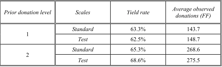
Table 2: Period 10 (Experiment) Average Donation Amounts and Frequencies
Prior donation level Scales Yield rate Average observed donations (FF)
1 Standard 63.3% 143.7
Test 62.5% 148.7
2 Standard 65.3% 268.6
[image:38.612.71.529.389.528.2]Table 3: Yield Rate and Average Amount of Observed Donations across Seasons
Level 1 Level 2
Easter June Christmas Easter June Christmas
Yield rate 71.9% 19.5% 21.7% 73.3% 20.1% 24.3%
Average donation per
occasion 139.1 125.3 126.9 258.8 217.2 206.6
Table 4: Proportion of Donations at Amounts* on Standard or Test Scales, Period 10
Level 1 Standard Level 1 Test Level 2 Standard Level 2 Test Scale
Point %
Scale
Point % p-value
Scale
Point %
Scale
Point % p-value 100* 18.6% 100 07.3% 0.000 100* 02.6% 100 01.6% 0.450
120 00.2% 120* 18.4% 0.000 120 00.1% 120* 02.9% 0.000 150* 17.8% 150 05.4% 0.000 150* 07.2% 150 01.8% 0.000 180 00.0% 180* 06.9% 0.000 200 02.6% 200* 18.8% 0.000 250* 05.1% 250* 04.4% 0.743 250* 026.7% 250 09.1% 0.000 350 00.0% 350* 00.3% 1.000 350 01.2% 350* 10.6% 0.000 500* 00.3% 500* 00.3% 1.000 500* 05.3% 500* 04.4% 0.627 1000* 00.0% 1000 00.0% 1.000 750 00.0% 750* 00.3% 1.000
None 49.4% None 50.2% 0.832 1000* 00.3% 1000 00.2% 1.000 Other 08.6% Other 06.8% 0.342 None 44.1% None 42.2% 0.618 Other 09.9% Other 08.1% 0.373
[image:39.612.70.553.373.625.2]Table 5: Parameter Estimates for Full Model
Coefficient mean SE 95% HDR
Homogeneo
u
s
correlation (ρ) -0.454 0.033 (-0.516, -0.385)
sd of log amount (σ) 0.299 0.004 (0.291, 0.307)
Easter dummy (βE) 0.708 0.026 (0.657, 0.757)
level dummy in selection (βlevel,s) 0.108 0.032 (0.047, 0.166)
log amount lag in selection (βlag) -0.123 0.006 (-0.136, -0.110)
level dummy in amount (βlevel,a) 0.260 0.013 (0.235, 0.287)
Heterogeneous
pulling up (βiU) -0.063 0.039 (-0.146, 0.007)
pulling down (βiD) 1.630 0.225 (1.245, 2.127)
June dummy (βiJ) -0.505 0.041 (-0.583, -0.425)
Christmas dummy (βiC) -0.993 0.049 (-1.090, -0.901)
sd of pulling up 0.330 0.022 (0.291, 0.378)
sd of pulling down 0.943 0.127 (0.726, 1.213)
sd of June 0.390 0.048 (0.308, 0.497)
sd of Christmas 0.777 0.060 (0.655, 0.895)
corr(June & Christmas) 0.714 0.083 (0.540, 0.871)
corr(pulling up & pulling down) 0.446 0.095 (0.243, 0.612)
corr(June & pulling up) -0.002 0.035 (-0.070, 0.065)
corr(June & pulling down) 0.002 0.035 (-0.066, 0.070)
corr(Christmas & pulling up) 0.003 0.034 (-0.064, 0.070)
Table 6: Model Fit Statistics (LPML, RMSE, MAD) for Various {IR, ER} Specifications and Restrictions, Computed over Model Posteriors
Internal Referent Specification (with ER-1) LPML RMSE MAD IR-1 (average of all prior donations) -21968 0.279 0.210 IR-2 (last donation) -22482 0.299 0.221 IR-3 (average of same-season donations) -22372 0.288 0.212 IR-4 (last same-season donation) -22558 0.294 0.222
IR-5: (geometrically smoothed, α = 0.4) -22125 0.277 0.207
IR-1 Model with Restrictions:
No correlation (ρ = 0) -22063 0.286 0.215
No scale effect -23095 0.335 0.226
Simple regression -23110 0.335 0.224 Heterogeneous scale effect only -22307 0.281 0.211 Heterogeneous seasonality only -22972 0.295 0.216 Homogeneous scale effect and seasonality -22716 0.297 0.218
Appendices A - C
A. Full Model Specification
As discussed above, we can write the entire model as follows (i = donor; t = time):
∗ ,
∗ , , where:
1, if ∗ 0; 0 otherwise
∗ ln , if 1; unobserved otherwise
;
∑ ,
1, , 1, ,
|| , ||
; exp ,
,
exp , , ,
|| , ||
, ~ 0, ; 1
~ ∆, , where , , ,
Note that the internal reference point, , for donor i can change over the course of the
experiment, and is subscripted accordingly, as is the kth external reference point for a donor i at
time t, , . Again, the variance of is fixed to 1 for identification. Finally, the vector of heterogeneous parameters ( ) follows a multivariate normal distribution with mean and