2018 IX International Conference on Optimization and Applications (OPTIMA 2018) ISBN: 978-1-60595-587-2
Multiobjective Optimization on Permutations with Applications
Liudmyla KOLIECHKINA
1,*and Oksana PICHUGINA
2,*University of Lodz, Uniwersytecka Str. 3, 90-137 Lodz, Poland
National Aerospace University Kharkiv Aviation Institute, Chkalova Str. 17, 61070 Kharkiv, Ukraine Corresponding author
Keywords: Multiobjective Combinatorial Optimization, Vector Optimization, permutation, structural graph, combinatorial configuration.
Abstract. A method of multiobjective optimization on permutations (MOP) is offered based on
the Directed Structuring Method and using Graph Theory. Prospects of applying graph techniques are caused by representability of the feasible domain by graph vertices. It yields advantages in using traditional methods, as well as in developing new ones. Our method is a generalization of the Method for Sequential Analysis of Variants for multiobjective optimization on permutations and multi-permutations. Most problems on combinatorial configurations sets are NP-hard, and a search of an exact solution requires enumerating a factorial number of variants. To decrease it, the method includes: a choice of an unconstraint MOP method; a choice of a method for generating a sequence of feasible solutions for a constraint MOP adapted to objective function; constructing and examining a structural graph of the optimization problem; a polynomial algorithm choice for solving the problem on partially ordered vertices of the graph.
Introduction
From the practical point of view, a wide and important class of decision-making problems is multiobjective problem, where the quality of a decision is evaluated regarding several criteria simultaneously [11, 12, 19].
Problems of optimization of several functions arise in the study of many theoretical and practical problems. Any problem of optimal design of complex economic and technical systems, schemes, technological devices, structures, scheduling, planning, and management of production activity, etc. requires the solution found takes into account many criteria and constraints [4–6,10, 23]. This problem is a multiobjective optimization one (MO problem, MP).
Research in the field of multiobjective optimization is currently intensively stimulated by prac- tical needs and development of computer information technology. This is the origin of a large number of papers devoted to MO [4–8, 10, 20, 23, 24].
In the simplest interpretation, MP includes objective functions and no additional constraints. When they are combined into a vector criterion, we come to a standard optimization problem. However, an adequate mathematical model of real-world problems includes several objective func- tions, as well as some additional constraints making it solving much more complicated than the simplest one.
In [4,6,7,10,20,22,25], methods for solving multiobjective optimization problems are considered, both constrained and unconstrained. In such studies [4, 6, 7, 10, 20, 22, 25], various approaches to
1
2
*
their solution are offered. In particular, methods of a search and examining the whole feasible domain are described in [4, 10, 20].
Since real-world systems are discrete-continuous by nature, they are modeled as partially inte-ger programs. In particular, numerous problems of planning, management, design, and placement are modeled with the help of multiobjective problems whose solutions are of combinatorial nature, e.g., permutations, partial permutations, combinations, compositions, partitions, as well as their composition images [5, 7, 8, 22–24]. In this case, the search for an optimal solution is conducted on the correspondent combinatorial set or its proper subset. MPs in their own are complex, but their solving becomes much more complicated if solutions are sought on a combinatorial set, and a multiobjective combinatorial optimization problem (a multiobjective combinatorial problem, a multiobjective CP, MCP) needs to be solved. MCP approaches take mainly are based on structural peculiarities of a particular combinatorial set. In [7, 8], a multiobjective optimization on permuta-tions without repetipermuta-tions is considered. The formulation of MCP on poly-partial permutapermuta-tions is formulated in [22, 23], and an approach to its solution using polyhedral relaxation is offered from the group of cutting methods. In [24], the MCP formulation of linear-fractional optimization is presented, and a solution method is offered, which is based on explored properties of a feasible combinatorial domain. A connection between the linear combinatorial optimization problem (lin-ear CP) and lin(lin-ear-fractional MCP is established for the case if the feasible domain is a set of combinations. It is well-known that standard combinatorial optimization methods typically are not applicable to problems with many criteria [22]. An advantage of the approach is that it allows applying classical optimization methods to solving MCP.
In studies [1–3], methods for solving CP are presented, which are based on the properties of graphs of polytopes of combinatorial sets. Such methods have advantages over classical ones. Since using the properties of the polytopes, the number of iterations (search operations) decreases, and the search itself is carried out along the vertices of the directed graph of the polytope, which vertex set represents the corresponding combinatorial set [2].
In [24], the MCP problem with a linear-fractional objective function on the set of permutations is solved by the coordinate method of localizing the value of a linear function for the solution of CP (the coordinate localization method, CLM). CLM is based on the construction of the CP graph and its decompositions into subgraphs and viewing a limited number of them.
Note that CLM was originally developed to a feasibility problem with an equality constraint. Adapted to a COP, CLM allows reducing significantly the number of combinatorial configurations considered [1, 3].
The goal of this paper is to develop a method for solving linear CP (LCP) on the general set of permutations [31] based on adapting CLM to the problem and to develop an approach to linear multiobjective optimization on the combinatorial set. For the case under consideration, CLM requires a modification (further referred to as a modified CLM (MCLM)) and development.
The extension from standard permutations without repetitions to multi-permutations, where a multiplicity of their components is permitted, allows covering a much wider class of MOPs, including boolean permutations appearing in modeling numerous graph problems [15]. Also, the method presented can be considered as a new approach to LCP on standard permutations. Also, the extension cover much wider class if LCPs than CLM.
The paper is organized as follows. In the second section, a multiobjective problem of Euclidean Combinatorial Optimization is formulated, and the conditions on the existence of a set of solutions are listed. Section 3 is dedicated to the analysis of methods and approaches to solving multicriteria
problems of this class. In Section 4, the structural graph of the optimization problem and its subgraph’s grids are presented, the method MCLM is described. In Section 5, two approaches to linear MCP (MLCP), based on applying MCLM, on the general set of permutations are outlined.
The Multiobjective Problem of Euclidean Combinatorial Optimization
MCP consists in optimizing several criteria{f1(x), f2(x), ..., fL(x)}on a finite setX, i.e., it can
be represented as:
(M CP)
fl(x)→min, l∈JL0 ={1, ..., L0};
fl(x)→max, l∈JL\JL0;
x∈X ⊆E0,
(1)
whereE0 is a combinatorial space,X is a set of feasible solutions, and the functions fl(x), l∈JL,
are defined on E0.
It is convenient to represent the criteria in the form of a vector function (a vector criterion)
F(x) ={fk(x), k∈JL}. As a result, (1) takes a form:
F(x)→extr, x∈X ⊆E0. (2)
Without loss of generality, we can assume that (2) has the form
(Z(F, X)) : F(x)→max, x∈X ⊆E0, (3) and F = (−f1(x), . . . ,−fL0(x), fL0+1(x), . . . , fL(x)). (4)
Note that each solution x= (x1, x2, ..., xn)∈X is characterized by a relevant vector estimate,
that is, a vectorF (x). Therefore, a choice of the optimal solution is, in fact, a choice of an optimal estimate from the set of estimates:
Y =F (X) =y∈RL
y=F (x), x∈X .
In this case, the effectiveness of the estimates (and solutions) is determined by a chosen principle of optimality.
Suppose that the combinatorial space E0 is a non-empty finite set of points Rn, and MCP
Z(F, X) with F = (f1, ..., fL) is considered. If a set E0 is an image of a certain set A of real
combinatorial objects in Euclidean space provided that between elements E0 and A a bijection is established, then the set A is Euclidean combinatorial set (e-set), and E0 is the correspond-ing set of Euclidean combinatorial configurations (C-set) [26]. Respectively, (3) belongs to the class of multiobjective problems of Euclidean Combinatorial Optimization (multiobjective ECOP, MECOP) [23, 26]. Moreover, it is a general mathematical model of MECOP.
Let us consider Z(F, X). Assume that a feasible domain X of the problem is non-empty and is can be represented as followsX ={x∈E ⊂Rn:x≥0, G(x)≤b} 6=
∅.This implies that there
exists a solution of the problem Z(F, G) for each component
fl(x), l∈JL, (5)
of a vector criterion F(X). Also, let us assume that the multiobjective problem Z(F, G) is such that extreme points xk of particular problems of optimizing (5) are not the same (otherwise, an
ideal solution of the problem exists). From this, it follows that a solution of the vector problem
Z(F, G) is a compromise satisfying in some way all components of the vector criterion. Therefore, solutions to the problems are not optimal, but effective.
To solve the problem of effective solution search, main affords in multiobjective optimization are directed [4–6, 11, 12, 19]. The first attempt to formulate a concept of effective solutions was done by V. Pareto (see, for instance, [12, 19]), and his set of such solutions is called Pareto set. However, when applying multiobjective methods, other effective solution sets can be more suitable. They can be restrictions of the Pareto set, as well as its extension. When applying one method of a multicriteria choice, Pareto set can be narrowed or expanded becoming Smale set, Slater set, etc. [12].
Under a solution ofZ(F, G) we mean an element or elements of one of the following sets [22–24]: 1. The setI(F, X) of ideal solutions:
I(F, X) ={x∈X :ν(x, F, X) = ∅},
where v(x, F, X) = {y∈X|∃l∈JL:fl(y)> li(x)};
(6)
2. Pareto set P(F, X), that is, sets of effective (optimal Pareto) solutions:
P(F, X) ={x∈X :π(x, F, X) = ∅},
whereπ(x, F, X) = {y∈X :F (y)≥F (x), F(y)6=F (x)}; (7)
3. Slater set Sl(F, X) of weakly effective solutions:
Sl(F, X) = {x∈X :σ(x, F, X) = ∅},
where σ(x, F, X) ={y∈X :F (y)> F(x)}; (8)
4. Smale set Sm(F, X) of strictly effective solutions:
Sm(F, X) = {x∈X :η(x, F, X) = ∅},
whereη(x, F, X) = {y∈X\ {x}:F (y)≥F (x)}. (9)
For instance, an element of the set (6) is called an ideal solution [4, 10, 23–25], and it is the best for all the particular criteria, respectively, for MP as well. At the same time, Pareto optimality (see (7)) means that the value of any of the particular criteria can be increased only by reducing the value of at least one of the other particular criteria. For a weakly effective estimate/solution (8) there will be no such estimate/solution that would be better with respect to all particular criteria. As a result, the sets (6)-(9) are connected as follows:
I(F, X)⊂Sm(F, X)⊂P(F, X)⊂Sl(F, X). (10)
It should be noted that, as a rule, when solving MPs, Pareto optimal solutions (effective solutions) are sought. We are not an exception.
Approaches to Multiobjective Euclidean Combinatorial Optimization
The problem of finding all effective solutions is not only of theoretical but also a great practical interest. It is explained by the fact that the construction of the whole Pareto set or its rather
broad subsets is one of the first stages in the whole series of optimal selection procedures under several criteria [10, 23, 24]. To solve the problem of constructing the set, one can choose two ways - to search directly on a feasible domain or to introduce a parametrizing set first and then search within it.
There are several directions of developing multiobjective optimization nowadays. Based on [4, 6, 10–12, 19, 22, 25], we offer the following typology:
methods based on convolution criteria into a single one;
methods based on imposing constraints on the criteria;
target programming;
methods based on finding a compromise solution;
methods based on man-machine procedures decision making (interactive programming). There are other ways of classifications of the methods, such as based on information available about the importance of criteria [12], etc.
When solving discrete multiobjective problems, a Pareto set formation requires a brute-force search. Thus, the way is intractable for large dimension problems. Taking into account the specifics of a problem is a very useful approach that enables to reduce the search significantly in many cases [5].
Majority of methods for constructing a set of effective solutions use certain optimality condi-tions. Most often, the necessary conditions are applied such as if a point is effective (in one or another sense, for example, according to one of the evaluation criteria (6)-(9)), then it is a solution to the problem (possibly with some additional constraints) of optimizing function of a special form with properly assigned parameters involving in this function and (or) constraints. Such a replace-ment of MP by a parametric family of standard optimization problems is called a scalarization of the original problem [22, 25]. If the optimality conditions are sufficient, then a set of solutions of the parametric problem is its effective solutions’ set. On contrary, a feasible set, constructed by means of scalarization, may contain extra points that should be identified and eliminated since the scalarization problem is, in most cases, is a relaxation to the original one. Thus, most common MO methods are the method of reducing MP to single-objective by convolution of a vector criterion into a super-criterion (further referred to as CM), the method of priorities, and their generalization - the method of successive concessions (further referred to as SCM) [10, 22, 25]. First one reduces the MP to a single-objective one, other two - to a sequence of single-objective problems.
In CM, a weighted sum of F(X)-components is considered as in a super criterion:
Φ(x) =
L X
l=1
αlfl(x), αl≤0, l∈JL0, αl ≥0, l∈JL\JL0, L X
l=1
|αl|= 1, (11)
and then the following problem is solved:
Φ (x)→max; x∈X ⊆E0 ⊂RN. (12)
When performing the convolution (11), the main issue and is a right choice of the coefficients
αl, l∈JL, the relative importance of the criteria implying that a solution x∗ of (3) coincide with
a solution x0 of (12) [10, 23].
By SCM [22], the individual criteria are ordered with respect to their relative importance
-fi1 fi2 ... fiL. Then the first, most important criterion, is maximized, and a constraint
fi1(x) ≥ f ∗
i1 −∆1 = f 0
i1 on lower bound of fi1(x) is added, where f ∗
i1 = minx∈Xfi1(x), ∆1 ≥ 0 - is
a concession on fi∗1. Next, the second most important criterion is optimized on a new domain
X1 ={x∈X : fi1(x)≥f 0
i1}, etc. As a result, a series of problems:
fil(x)→max, x∈X
l−1 ⊆E0
, l∈JL, (13)
where X0 =X,
Xl ={x∈Xl−1 :fil0(x)≥f 0 i0l, l
0 ∈
Jl−1},
fi0
l =f
∗
il−∆l, f
∗
il = min
x∈Xl−1fil(x), ∆l≥0, l ∈JL−1.
(14)
x∗ is obtained as a solution of last of them.
If (3) is MECOP, problems (12), (13) are MCPs, which can be solved effectively using a specifics of the problem, in particular, taking into account properties of a particular Euclidean combinatorial set and the behavior of objective functions on it [22, 25–27, 31].
For instance, if MCP is linear, that is both functions (5) and constraints that single out X
from E0 are linear, then the problems (12), (13) are linear ECOPs, which can solved by methods of combinatorial cuttings [17, 32] and other specific techniques [30].
The practice has shown that the majority of ECOPs is posed on the sets of Boolean vectors or permutations [9, 13–15, 21]. This implies that typically E0 is the basic Boolean C-set (Cb-set)
Bn of n-dimensional Boolean vectors or the general Cb-set of permutations Enk(G) induced by
n-element numerical multisetG={g1, ..., gn}, g1 ≤. . .≤gn, containing k different elements [26].
A particular case of MO on Enk(G) considered by now corresponds to k =n, where G - is a set.
It is En(G) calledCb-set of permutations without repetitions or simply Cb-set of permutations. An
interesting feature of such ECOPs is thatE0, and accordingly X, coincides with the set of vertices of its convex hull:
E0 =vert P0, P0 =conv E0.
Thus, E0 is vertexlocated [26, 31]. Also, both of these sets are inscribed into hyperspheres
-∃x0 ∈
Rn, ∃r∈R1+ : (x−x0) 2
=
E0r 2,
E ∈ {Enk(G), Bn}. (15)
This means, they both are spherically-located [16, 17, 26, 29].
From this, it follows that MECOP (3), (15) allows reformulating in the form of a continuous MP as follows [15, 29]:
F(x)→max, (16)
x∈P0 ∩Sr(x0), hi(x)≤0, i∈Jm, (17)
where P0, Sr(x0) are represented in an analytic form, hi(x) ≤ 0, i ∈ Jm, - are constraints that
single out X fromE0.
Respectively, the MCP is reformulated as a multiobjective global optimization problem. It can be solved by means of nonlinear optimization. Moreover, (16), (17) allows assuming that
F(x), hi(x), i∈Jm, - are convex [18, 29, 31], thus, convex optimization techniques are applicable
to such MECOP as well.
Another equivalent formulation of MECOP is related to the possibility of representing it as a problem on vertices of a geometric graph G = (E0,E), E=edgesP0, which is a skeleton graph of
P0 and has the form (16),
x∈E0 ⊂Rn, h
i(x)≤0, i∈Jm.
To this formulation, different graph techniques become applicable [1–3], which can be combined with properties of the Euclidean space [26]. Finally, the graphGcan be complemented by additional edges decreasing diameter of theG∗ = (E0,E∗) (further referred to as an auxiliary graph),E∗ ⊃E.
In turn, forming a directed graph fromG∗ based on a specifics of ECOP allows applying techniques
from [2, 3].
Further, we focus on the case E0 =Enk(G), thus, the problem (16),
x∈Enk(G), hi(x)≤0, i∈Jm (18)
(further referred to as MCPP) will be considered, and the corresponding ECOP (12), (18) (further referred to as CPP). Consequently, the constraint problem on the generalizedCb-set of permutations
is considered.
CPP is a discrete optimization problem solvable by relevant methods such as branch-and-bound, cutting, branch and cuttings, etc. [9, 21]. Here should also be noted the method of directed structuring CLM described in [1–3] are highly promising for solving such a class of problems.
We study the vector optimization problems on a combinatorial set of permutations and offer a method for solving such problems using Graph Theory, which take into account structural and geometric properties the set of permutations.
The Modified Coordinate Localization Method (MCLM)
CLM was original developed to solve a feasibility problem - to find x ∈ En(G) satisfying
equalityf(x) =aTx−b = 0 [1, 3]. It uses a reformulation of the problem as CPP (further referred
as CPP1):
f(x)→max; x∈Enk(G);f(x)≤0.
For CPP1, CLM uses its representation in the form of a directed graph, where the direction of arcs corresponds to the increasing values of the objective function. An important issue is that the usage of above reformulation allows performing a search within a feasible domain of CPP1
-D={x∈Enk(G);f(x)≤0} and move towards its solution from a minimizer of f to a minimizer.
When implementing the method, branching and estimate evaluating, based on the examining a feasible domain X as a subset Enk(G), are performed allowing to prune a part of the branches.
To a particular CPP, a structural graph G0 (further referred to as SG) is associated, which is
constructed from the auxiliary graph G∗. In turn,G∗ is formed on the basis of a skeleton graphG
of the generalized permutohedron P0 =Pnk(G). Its important feature of SG is that, when solving
an optimization problem, the only a part of vertices associated with elements of X is analyzed, thus, avoiding a brute-force search.
A skeleton graphG ofP0 has edges (u, v) wheneveru, v ∈E0 =Enk(G) are differ by an adjacent
transposition. It is a subgraph ofG∗, for whichu, v ∈E0 are adjacent whenever u, v ∈E0 are differ
by a transposition. A necessity to consider the auxiliary graph instead of G is caused by our goal to solve MPP examining a part of the graph vertex set and moving along its edges. To understand
the difference between G, G∗, let us compare their degrees of vertices. d G =
k−1 P
i=1
nini+1, where ni
- is a multiplicity of ei, i ∈ Jk−1, S(G) = {e1, ..., ek} is a ground set of G, e1 < . . . < ek. At the
same time, dG∗ = P 1≤i<j≤k
nini+1.
The auxiliary graph G∗ can be constructed by applying a series of the following method of
generating E0 [2] and formingE from the obtained Hamiltonian paths.
A scheme of a recursive construction method of G∗:
1. SetE=∅, κ=k;
2. Start from the pointx=g = gi1, ..., gin−1, eκ
∈E0. Assign i=n.
3. Fix an item with an indexi in the sequence of coordinates of the current point x. The rest
i−1 elements are generated as follows:
(a) moving from left to right, find the lowest position where gi > gi+1;
(b) look for the smallest elementgj located on the left and smaller than it;
(c) make a transposition of elements gj and gi getting y∈E0;
(d) E=E∪ {x, y};
4. Assignx=y, i=i−1. If i≥1, go to Step 3. 5. Setκ=κ−1. If κ≥1, go to Step 2.
Remark 1. If G = Jn, E0 turns into a standard set of permutations En = En(G). Further, we
mostly consider this case.
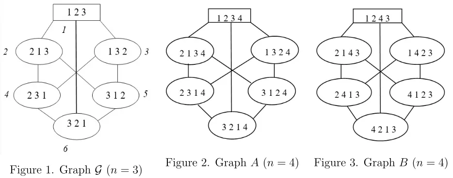
Figure 1. GraphG (n= 3) Figure 2. GraphA (n = 4) Figure 3. Graph B (n= 4)
Now, consider in details a structure of the auxiliary graphs G∗
n = G∗ for n = 3,4, E0 = En.
Fig.1 depicts the graph G3∗. For n = 4, four graphs A, B, C, D isomorphic to G3∗ is associated. Therefore, they can be formed from G∗
3. For instance, the subgraph A with x4 = 4 is presented in
Fig. 2 and formed fromG∗
3 by adding 4 to the labels on the right. The subgraph B corresponds to
x4 = 3 and is shown in Fig. 3. It can be obtained from Fig. 2 by substitutions 3→4, 4→3 in the
labels. Similarly, the remaining graphs C, D are constructed fixing 2 and 1 on the last position, respectively.
[image:8.612.74.541.447.631.2]Note that in the subgraphs of G∗
4, the place of the last element is uniquely determined. In
general, for G∗
n, all the subgraphs Gi, i ∈ Jn are copies (projections) of subgraph Gn∗−1, and they
can be ordered by the value of the last coordinate of its vertices. In turn,Gi, i∈Jn, are connected
by edges of other partitions of E0 by n subgraphs corresponding to fixing coordinates other than
xn.
In the general case of E0 =Enk(G), the partition will be made by k subgraphs corresponding
to a fixed coordinate i ∈Jn. In general, these subgraphs are not isomorphic, and their structure
is completely determined by multiplicities of inducing multisets [26].
This partition of G∗ provides the possibility of constructing special graph methods of
combi-natorial optimization on the set En(G), which was used in studies [2, 3].
Let CPP2 be the following single-objective constraint program
f(x)→max; x∈E0 =Enk(G);hi(x)≤0, i∈Jm,
and hx∗, f∗i - be its solution.
Definition 1. A directed graph G0 = (V0,E0) is called a structural graph (SG) of CPP1, if it satisfies the following conditions: a) X = V0; b) E0 ⊆ E∗; ∀x, y ∈ X, if {x, y} ∈ E∗, then: a) if
f(x)≤f(y), then an arc (x, y)∈E∗; b) if f(x)≥f(y), then (y, x)∈E∗.
Thus, SGG0 is a graph of the feasible domain of CPP2, where directions of arcs correspond to increasing of f(x).
Let the following linear CPP2 (further referred to as LCPP) is considered:
f(x) =aTx→max; (19)
hi(x) =aiTx−bi ≤0, i∈Jm; (20)
where a1 ≥a2 ≥...≥an, (21)
xmin =argmin
x∈E0f(x)∈X. (22)
Now we present a generalization of CLM for solving CPP2. CLM was developed for solving a specific problem of this class with an equality-constraint [1, 3]. For the generalization of CPP1, we add the condition (22), and it is the only restriction in comparison with a general LCP on sets of this class. It is added in order to use the same idea as CLM, namely, performing a search within a feasible domain. According to (21) and well-known properties of linear function on Enk(G), (22)
can be rewritten in the form
xmin =g = (g
1, ..., gn)∈X. (23)
LCPP is solved to optimality, if
xmax =argmax
x∈E0f(x) = (gn, ..., g1), (24)
wherefrom x∗ = xmax. In case if (24) does not hold, we organize a directed search of x∗ on G0
based on the decomposition of G0 into directed subgraphs, similar to those presented earlier for
G∗.
Let us fixQ≤n−3 and choose Λ = (λq)q∈JQ ⊂Jn. To Λ, a graph G
0(Λ), which is an induced
subgraph of G0, is associated, such as
G0(Λ) = (X(Λ), E(Λ))⊆G0 :X(Λ) = {x∈X :xn−q+1 =gλq, q∈JQ}. (25)
Similarly, induced subgraphs G(Λ)⊆ G,G∗(Λ) = (V(Λ), E∗(Λ))⊆ G∗, whereV(Λ) ={x∈E0 :
xn−q+1 =gλq, q∈JQ} can be defined by eliminating from their vertex sets those vertices, who do
not satisfy the constraints:
xn−q+1 =gλq, q∈JQ. (26)
Consider a set Ψ = {Λ ⊂ Jn : |Λ| = Q}. It is a cover of Jn by AQn subsets, where AQn is the
number of Q-permutations out of n. The cover Ψ induces a partition of G into AQn subgraphs of type (25). A structure of a permutation graph G is such that, for any Λ∈ Ψ, a graph G(Λ) is a permutation graph of E0(Λ) as well, and its dimension is n−Q. Here,
E0(Λ) =En−Q,k(Λ)(G(Λ)), G(Λ) =G\{gλq}q∈JQ,
k(Λ) is a cardinality of a ground set of G(Λ). In particular, if E0 = En(G), then
E(Λ) = En−Q,k−Q(G(Λ)), thus, all the subgraphs are isomorphic to Gn−Q. The same holds for G∗(Λ). Respectively, G0(Λ) are structural graph of the corresponding LCPP (further referred as
LCPP(Λ)) - (19)-(21), (26). LCPP is a particular case of LCPP(Λ), namely, LCPP(∅)=LCPP(Λ). So, for arbitrary LCPP(Λ), (23) and (24) are generalized as follows:
xmin(Λ) =arg min
x∈E0(Λ)f(x) = (gµ1, ..., gµn−Q, gλQ, ..., gλ2, gλ1); (27)
xmax(Λ) =arg min
x∈E0(Λ)f(x) = (gµn−Q, ..., g1, gλQ, ..., gλ2, gλ1), (28)
where {µi}i∈Jn−Q =Jn\Λ,gµ1 ≤...≤gµn−Q.
A fixation ofQ, which does not depend onn, induces a partition ofG0 into a polynomial number of subgraphs Ω = {G0(Λ)}Λ∈Ψ, similar to the original one. They induce branches of a search tree
of LCPP. Now, if a search ofx∗ is organized in such a way that for examining Ω-components, it is sufficient to consider a polynomial number of points, the problem will be polynomially solvable.
The search will be organized as follows.
MCLP for LCPP2
.
Input: LCPP2. Output: hx∗, z∗i. An algorithm:
Step 1. ChooseQ, form the family Ψ. Set x∗ =g, z∗ =cTg;
Step 2. For each Λ∈Ψ, verify:
– if xmin(Λ) does not satisfy (20), then LCPP(Λ) is infeasible;
– ifxmax(Λ) satisfy (20), it is a solution of LCPP(Λ). Ifz∗ < zmax(Λ) =cTxmax(Λ), then
setx∗ =xmax(Λ), z∗ =zmax(Λ);
– otherwise, apply a search within a family of subgraphs-grids (see Algorithm 1), choosing as a starting pointxmin(Λ)∈X according to (27).
Definition 2. For E = En(G), a grid Gr(Λ) of a subgraph of G0(Λ) is a grid of the dimension
(n−Q−1)×(n−Q) with the following properties:
its node set N odes(Λ) = {pij}i∈Jn−Q−1,j∈Jn−Q ⊆E
0; its top-left node (a source) is (27) - p1,1 =xmin(Λ);
last Q coordinates are fixed;
from left to right, n−Q-th coordinate of nodes decreases gradually from gµn−Q togµ1, and
first n−Q−1 coordinates are ordered decreasingly;
from top to bottom,n−Q-th coordinate of nodes is fixed,n−Q−1-th coordinate decreases gradually from its original value to gµ1, and the first n− Q−2 coordinates are ordered
decreasingly.
As a result, a bottom-right node (a sink) pn−Q−1,n−Q will have gµ2, gµ1 on last two positions,
respectively.
Let us introduce a lexicographic order on the grid’s nodes in the following way:
∀pij, pi0j0 ∈N odes(Λ) pij pi0j0 ⇔f(pij)≤f(pi0j0),
and formulate an important statement in terms of the lexicographic order.
Theorem 1. If Λ∈Ψ then for Gr(Λ) it is true:
∀i∈Jn−Q−2, j ∈Jn−Q pij pi+1,j, pij, pi+1,j are differ by a transposition; ∀i, j ∈Jn−Q−1 pij pi,j+1; pij, pi,j+1 are differ by a transposition.
Corollary 1.
∀i∈Jn−Q−2, j ∈Jn−Q: (pij, pi+1,j)∈E∗(Λ); if pij, pi+1,j ∈X, then (pij, pi+1,j)∈E(Λ); ∀i, j ∈Jn−Q−1, (pij, pi,j+ 1)∈E∗(Λ); ifpij, pi,j+1 ∈X, then (pij, pi,j+1)∈E(Λ);
Corollary 2.In a sink of Gr(Λ), it is attained a maximum of f on the grid:
f(pn−Q−1,n−Q) = max pij∈N odes(Λ)
f(pij).
Theorem 1 means that we perform a directed search of x∗ examining N odes(Λ) from left to right and from top to bottom. Corollary 1 implies that neighboring nodes inGr(Λ) are adjacent in
G∗, and the direction of the arcs is uniquely determined by indexes of the nodes. Finally, Corollary
2 says that for examining Gr(Λ) it is sufficient to check the only pn−Q−1,n−Q, if this node is inX.
To decrease the number of nodes examined, the following statement ca be applied.
Theorem 2. If Λ∈Ψ then for Gr(Λ)-nodes it is true:
∀i∈Jn−Q−1, if ∃j0 ∈Jn−Q−1 pij0 ∈X, pi,j0+1 ∈/ X, then pi,j ∈/ X, j > j0+ 1; ∀i, j ∈Jn−Q−1, if ∃i0 ∈Jn−Q−2 pi0j ∈X, pi0+2,j0 ∈/ X, then pi,j ∈/ X, i > i0+ 1.
Let
xmin(Gr(Λ)) = arg min
x∈E0(Λ)∩Gr(Λ)f(x),
xmax(Gr(Λ)) =arg max
x∈E0(Λ)∩Gr(Λ)f(x).
By construction, xmin(Gr(Λ))∈X, hence, by (27),
xmin(Gr(Λ)) =xmin(Λ) = (g
µ1, ..., gµn−Q, gλQ, ..., gλ2, gλ1).
At the same time,
zmax(Gr(Λ)) =f(xmax(Gr(Λ))≥f(xmin(Λ)), (29)
where xmin(Λ) is given by (28).
Algorithm 1 of examining Gr(Λ) and a search of x∗0 =xmax(Gr(Λ)), z∗0
=f(x∗0).
Step 1. Set x∗0 =xmin(Λ), z∗0 =f(x∗0);
Step 2. Check xmax(Gr(Λ))∈X, thenx∗0
=xmax(Gr(Λ)),z∗0
=zmax(Gr(Λ)), finish;
Step 3. Moving along rows from left to right or from top to bottom, examine a part of Nodes(Λ) according to Theorem 2, and improving z∗0 and updating x∗0 as far as new nodes inX are found.
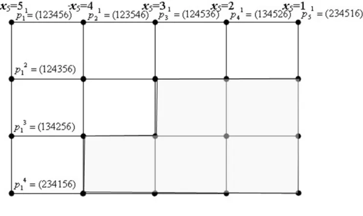
In Fig. 4, it is shown a grid Gr1 = Gr(Λ) for G = Jn, n = 6, Q = 1, Λ = {6}. Here,
a source is g = (1,2,3,4,5,6,7), and a sink is xmax(Gr(Λ)) = (3,4,5,2,1,6), unfeasible nodes of the grid is shadowed. It is clear that, here, (29) is fulfilled as a strict inequality, and
xmax(Gr(Λ))6=xmax(Λ) = (5,4,3,2,1). Thus, the only partial examination of G0(Λ) is performed
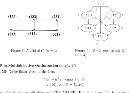
byGr(Λ). On the other hand, Figure 5 depicts a gridGr2 =Gr(Λ) forG=Jn, n = 3, Q= 0,Λ =∅,
wherexmax(Gr(Λ)) = xmax(Λ) = (3,2,1). Now, examiningGr(Λ) is equivalent to the one ofG0(Λ).
In Fig. 6, it is shown a directed graph G∗∗
3 , which is isomorphic to G ∗
3 and is associated to Gr2,
wherefrom it is seen, why a G-consideration is nor sufficient for the subgraph-grid approach to LCPP2.
Thus, only provided the choice Q=n−3 (casesn = 1,2 are evident), MCLM allows obtaining
x∗, while requires examining a non-polynomial number of subgraphs and grids, namely, Ann−3 =
n!/3. At the same time, choosing a fixed Q, the scheme allows obtaining an approximate solution of CPP2 in polynomial time onn. Depending on accuracy, we wish to achieve and time available,
Q can be chosen closer ton−3 or to 0.
[image:12.612.121.492.434.655.2]Thus, presenting MLCM, we offer a flexible approach to solve LCPP2 including as greedy algorithms for Q < n−3, as well as a brute force search type forQ=n−3.
Figure 4. A subgraph grid (n= 6)
Remark 2. If MLCM is applied to LCPP on Enk0 (G), where k < n, the subgraph-grids are rectangular as well. However, some adjacent nodes of the grids may correspond to the same point of E0. Also, the grid dimensions depend on Q, n, K,Λ and do not exceed (n−Q−1)×(n−Q).
Figure 5. A grid ofG0 (n = 3) Figure 6. A directed graph G∗∗
(n = 3)
MLCP in Multiobjective Optimization on Enk(G)
Let MP (2) be linear given in the form
fl(x) =a 0T
l x→max, l∈JL;
s.t.(20), x∈E0 =Enk(G)
(further referred to as a multiobjective LCPP, MLCPP). If m = 0, hence (20) is absent, it is an unconstrained MLCPP, otherwise, - a constrained MLCPP.
Choosing coefficients of the relative importance of criteria (30) and applying a convolution to them in accordance to (11), (12), we get a linear CPP with f(x) = Φ(x). If, in addition, (22) holds, it is LCPP, to which MLCP is applicable directly. In particular, unconstrained MLCPPs will always be solved on the second stage of MLCP.Step 2.
To unconstrained MLCPP, MLCP can be used in SCM as well. For that, in (14), values of concession ∆l ≥ 0, l ∈ JL−1, need to be chosen such that to presume fulfillment of conditions,
similar to (22) on each iteration. Namely,
xl,min=argmin
x∈E0fl(x)∈X
l−1, l∈J L−1.
Conclusions and Future Research
In the paper, the modified coordinate localization method (MLCM) is presented. It generalizes the coordinate localization method (CLM) to the whole class of constrained linear programs on sets of Euclidean configurations of permutations, to an arbitrary finite number of inequality constraints, and with a minor restriction. Two approaches to multiobjective linear optimization on these combinatorial sets are described, implementing MLCM, the convolution and successive concessions methods to multicriteria optimization on permutations, Boolean permutations, and other classes of multi-permutations.
MLCM and the multiobjective approaches may be extended and generalized to solve multiob-jective problems on other classes vertex-located C-sets [13, 15, 16, 26, 28]
References
[1] G. A. Donec and L. M. Kolechkina. Construction of hamiltonian paths in graphs of permu-tation polyhedra. Cybernet. Systems Anal., 46(1):7–13, 2010.
[2] G. A. Donets and L. M. Kolechkina. Extremal problems on combinatorial configurations. RVV PUET, 2011.
[3] G. A. Donets and L. N. Kolechkina. Method of ordering the values of a linear function on a set of permutations. Cybern Syst Anal, 45(2):204–213, 2009.
[4] Matthias Ehrgott. Multicriteria Optimization. Springer, 2nd edition, 2005.
[5] Matthias Ehrgott and Xavier Gandibleux. Multiobjective combinatorial optimization — the-ory, methodology, and applications. In Matthias Ehrgott and Xavier Gandibleux, editors,
Mul-tiple Criteria Optimization: State of the Art Annotated Bibliographic Surveys, number 52 in
International Series in Operations Research & Management Science, pages 369–444. Springer US, 2003.
[6] Matthias Ehrgott and Margaret M. Wiecek. Mutiobjective programming. InMultiple Criteria
Decision Analysis: State of the Art Surveys, number 78 in International Series in Operations
Research & Management Science, pages 667–708. Springer New York, 2005.
[7] L. M. Koliechkina and O. A. Dvirna. Solving extremum problems with linear fractional objective functions on the combinatorial configuration of permutations under multicriteriality.
Cybern Syst Anal, 53(4):590–599, 2017.
[8] L. N. Koliechkina, O. A. Dvernaya, and A. N. Nagornaya. Modified coordinate method to solve multicriteria optimization problems on combinatorial configurations. Cybern Syst Anal, 50(4):620–626, 2014.
[9] Bernhard Korte and Jens Vygen. Combinatorial Optimization: Theory and Algorithms. Springer, 5th edition, 2012.
[10] Massimo Pappalardo. Multiobjective optimization: A brief overview. In Altannar Chinchu-luun, Panos M. Pardalos, Athanasios Migdalas, and Leonidas Pitsoulis, editors, Pareto
Opti-mality, Game Theory And Equilibria, number 17 in Springer Optimization and Its
Applica-tions, pages 517–528. Springer New York, 2008.
[11] Panos M. Pardalos, Antanas ˚A½ilinskas, and Julius ˚A½ilinskas. Non-Convex Multi-Objective
Optimization. Springer Optimization and Its Applications. Springer International Publishing,
2017.
[12] A.B. Petrovsky. Decision Making Theory. Publishing Center Academiya, 2009.
[13] O. Pichugina. Placement problems in chip design: Modeling and optimization. In 2017 4th International Scientific-Practical Conference Problems of Infocommunications Science and
Technology, PIC S and T 2017 - Proceedings, pages 465–473, 2017.
[14] O. Pichugina and B. Farzad. A human communication network model. In CEUR Workshop
Proceedings, pages 33–40, 2016.
[15] O. Pichugina and S. Yakovlev. Convex extensions and continuous functional representations in optimization, with their applications. J. Coupled Syst. Multiscale Dyn., 4(2):129–152, 2016. [16] O. Pichugina and S. Yakovlev. Optimization on polyhedral-spherical sets: Theory and ap-plications. In 2017 IEEE 1st Ukraine Conference on Electrical and Computer Engineering,
UKRCON 2017 - Proceedings, pages 1167–1174, 2017.
[17] O. S. Pichugina. Surface and combinatorial cuttings in euclidean combinatorial optimization problems. Math. and Comp. Model., Ser. Phys. and Math., 1(13):144–160, 2016.
[18] O. S. Pichugina and S. V. Yakovlev. Continuous representations and functional extensions in combinatorial optimization. 52(6):921–930.
[19] V.V. Podinovskii and V.D. Noghin. Pareto-optimal Decisions in Multicriteria Optimization
Problems. Nauka, 2 edition edition, 2007.
[20] El-Desouky Rahmo and Marcin Studniarski. Generating epsilon-efficient solutions in mul-tiobjective optimization by genetic algorithm. Discrete Applied Mathematics, (8):395–409, 2017.
[21] Alexander Schrijver. Combinatorial Optimization: Polyhedra and Efficiency. Springer Science & Business Media, 2012.
[22] N. V. Semenova and L. M. Kolechkina. Vector problems of discrete optimization on
combina-torial sets: methods of research and solution. Naukova Dumka, 2009.
[23] N. V. Semenova, L. M. Kolechkina, and A. M. Nagirna. Multicriteria lexicographic optimiza-tion problems on a fuzzy set of alternatives. Dopov. Nats. Akad. Nauk Ukr. Mat. Prirodozn.
Tekh. Nauki, (6):42–51, 2010.
[24] N. V. Semenova, L. N. Kolechkina, and A. N. Nagornaya. On an approach to the solution of vector problems with linear-fractional criterion functions on a combinatorial set of arrange-ments. Problemy Upravlen. Inform., (1):131–144, 2010.
[25] Ralph E. Steuer. Multiobjective programming. In Saul I. Gass and Michael C. Fu, editors,
Encyclopedia of Operations Research and Management Science, pages 996–1003. Springer US,
2013.
[26] Yu G. Stoyan, S. V Yakovlev, and O. S. Pichugina. The Euclidean combinatorial
configura-tions: a monograph. Constanta, 2017.
[27] S. Yakovlev, O. Pichugina, and O. Yarovaya. On optimization problems on the polyhedral-spherical configurations with their properties. In 2018 IEEE First International Conference
on System Analysis & Intelligent Computing (SAIC2018)- Proceedings, pages 94–100.
[28] S. V Yakovlev and O. S. Pichugina. Optimization problems over euclidean combinatorial con-figurations and their properties. Problems of applied mathematics and mathematical modeling, (17):278–263, 2017.
[29] S. V. Yakovlev and O. S. Pichugina. Properties of combinatorial optimization problems over polyhedral-spherical sets. Cybern. Syst. Anal., 54(1):99–109, 2018.
[30] S. V. Yakovlev and O. A. Valuiskaya. Optimization of linear functions at the vertices of a permutation polyhedron with additional linear constraints. 53(9):1535–1545.
[31] Sergey Yakovlev. Convex extensions in combinatorial optimization and their applications. In
Optimization Methods and Applications, Springer Optimization and Its Applications, pages
567–584. Springer, Cham, 2017.
[32] Oleg A. Yemets, Yelizaveta M. Yemets, and Tatyana V. Chilikina. Combinatorial cutting while solving optimization nonlinear conditional problems of the vertex located sets. JAI(S), 42(5):21–29, 2010.