Comparison of hierarchical cluster analysis methods by cophenetic correlation

(1)

R E S E A R C H

Open Access

Comparison of hierarchical cluster analysis

methods by cophenetic correlation

Sinan Saraçli

1*

_{, Nurhan Do ˘gan}

2

_{and ˙Ismet Do ˘gan}

2

*_{Correspondence:}

[email protected]

1_{Department of Statistics, Faculty of}

Arts and Sciences, Afyon Kocatepe University, Afyonkarahisar, 03200, Turkey

Full list of author information is available at the end of the article

Abstract

Purpose:This study proposes the best clustering method(s) for different distance measures under two different conditions using the cophenetic correlation coefficient.

Methods:In the ﬁrst one, the data has multivariate standard normal distribution without outliers forn= 10, 50, 100 and the second one is with outliers (5%) for

n= 10, 50, 100. The proposed method is applied to simulated multivariate normal dataviaMATLAB software.

Results:According the results of simulation the Average (especially forn= 10) and Centroid (especially forn= 50 andn= 100) methods are recommended at both conditions.

Conclusions:This study hopes to contribute to literature for making better decisions on selection of appropriate cluster methods by using subgroup sizes, variable numbers, subgroup means and variances.

Keywords: cophenetic correlation; hierarchical clustering methods; distance measures

1 Introduction

Classiﬁcation, in its widest sense, has to do with forms of the relatedness and with the organization and display of the relations in a useful manner. The items to be studied could be anything: people, bacteria, religions, books,etc.The attributes in each case would be those features of the items that are of interest for the purpose of the study []. Classiﬁ-cations are generally pictured in the form of hierarchical trees, also called a dendrogram. A dendrogram is the graphical representation of an ultrametric (= cophenetic) matrix; so dendrograms can be compared to one another by comparing their cophenetic matrices []. Cluster Analysis (CA), Principal Components Analysis (PCA) and Discriminant Analy-sis (DA) are three of the primary methods of modern multivariate analyAnaly-sis. Because of its utility, clustering has emerged as one of the leading methods of multivariate analysis [].

Cluster analysis is a multivariate statistical technique which was originally developed for biological classification. Biologists Robert Soka and Peter Sneath published their semi-nal text ‘Principles of Numerical Taxonomy’ in . Sokal and Sneath demonstrated that cluster analysis could be utilized to efficiently classification a data set which contained all relevant characteristics of an organism. When the organisms had been classified based on these characteristics, it could be determined in which way they differed, and if they be-longed to different species. In this way, Sokal and Sneath asserted, researchers could trace the path of evolution from one species to another [].

(2)

In this study for clustering, two measures of cluster ‘goodness’ or quality are used. One type of measure allows us to compare diﬀerent sets of clusters without reference to ex-ternal knowledge and is called an inex-ternal quality which is used as a measure of ‘overall similarity’ based on the pairwise similarity of documents in a cluster. The other type of measures allows evaluating how well the clustering is working by comparing the groups produced by the clustering techniques to known classes. This type of measure is called an external quality measure, which is not scope of this study [].

The joining or tree clustering method uses the dissimilarities (similarities) or distances (Euclidean distance, squared Euclidean distance, city-block (Manhattan) distance, Cheby-chev distance, power distance, Mahalanobis distance,etc.) between objects when forming the clusters. Similarities are a set of rules that serve as criteria for grouping or separat-ing items. These distances (similarities) can be based on a sseparat-ingle dimension or multiple dimensions, with each dimension representing a rule or condition for grouping objects. The joining algorithm does not ‘care’ whether the distances that are ‘fed’ to it are actual real distances, or some other derived measure of distance that is more meaningful to the researcher; and it is up to the researcher to select the right method for his/her speciﬁc application [].

The next step is to identify how one can ﬁnd the natural clusters among items char-acterized by many attributes. A number of cluster analysis procedures (single linkage (nearest neighbor), Complete linkage (furthest neighbor), Unweighted pair-group aver-age (UPGMA), Weighted pair-group averaver-age (WPGMA), Unweighted pair-group centroid (UPGMC), Weighted pair-group centroid (median), Ward’s method, etc.) are available; many of these begin with ann-dimensional space in which each entity is represented by a single point. The dimensions in the space represent the characteristics upon which the entities are to be compared. Similarity between entities can be measured by: () the cor-relation of entities’ scores on the dimensions (cophenetic corcor-relation) or () the distance between points in the space (points closest to each other are most similar) [, ].

Suppose that the original data{Xi}have been modeled using a cluster method to

pro-duce a dendrogram{Ti}; that is, a simpliﬁed model in which data that are ‘close’ have been

grouped into a hierarchical tree. Deﬁne the following distance measures.x(i,j) =|Xi–Xj|,

the ordinary Euclidean distance between theith andjth observations.t(i,j) = the dendro-grammatic distance between the model pointsTiandTj. This distance is the height of the

node at which these two points are ﬁrst joined together. Then, lettingxbe the average of thex(i,j), and lettingtbe the average of thet(i,j), the cophenetic correlation coeﬃcientc

is deﬁned as in () [].

c=

i<j(x(i,j) –x)(t(i,j) –t)

[_i_<_j(x(i,j) –x)_][

i<j(t(i,j) –t)]

. ()

(3)

assess cluster-based models of DNA sequences, or other taxonomic models), it can also be used in other ﬁelds of inquiry where raw data tend to occur in clumps, or clusters. This coeﬃcient has also been proposed for use as a test for nested clusters [].

The problem of comparing classifications with numerical methods is not new; the first effective numerical method known to us is the ‘cophenetic correlation’ technique of Sokal and Rohlf []. Beginning with the development of cophenetic correlations methods for comparison of dendrograms have recently been the object of strong interest. Baker [] investigated the impact of observational errors on the dendrograms produced by the com-plete linkage and single linkage hierarchical grouping techniques. The goodness of fit of the dendrograms was measured by means of the Goodman-Kruskal gamma coefficient. The gamma coefficients indicated that the single linkage grouping technique was more sensitive to the type of data errors employed than the complete linkage technique. Hu-bert [] compared two rank orderings of the object pairs. He tested hypothesis that the given set of proximity values have been assigned randomly by referring the Goodman-Kruskal rank correlationγ statistic to an approximate permutation distribution. Kuiper and Fisher [] compared six hierarchical clustering procedures (single linkage, complete linkage, median, average linkage, centroid and Ward’s method) for multivariate normal data, assuming that the true number of clusters was known. The authors used the Rand index, which gives a proportion of correct groupings, to compare the clustering methods. In their study for clusters of equal sizes, Ward’s method and complete linkage method, with very unequal cluster sizes centroid and average linkage method found best, respec-tively. Blashfield [] compared four types of hierarchical clustering methods (single link-age, complete linklink-age, average linkage and Ward’s method) for accuracy in recovery of original population clusters. He used Cohen’s statistic to measure the accuracy of the clus-tering methods. According to his results, Ward’s method performed significantly better than the other clustering procedures and average linkage gave relatively poor results. Ac-cording to Milligan [], complete linkage and Ward’s method reacted badly when outliers were introduced into the simulated data.

(4)

Consider the studies in the literature and the importance of using the most convenient cluster method under different conditions (sample size, variables number and distance measures), a detailed simulation study is undertaken. This study gives more insight into the functioning of the cluster method under different conditions. The purpose of this re-search is to investigate the best clustering method under different conditions.

2 Method

In this study, seven cluster analysis methods are compared by the cophenetic correlation coeﬃcient computed according to diﬀerent clustering methods with a sample size (n= ,

n=  andn= ), variables number (x= ,x=  andx= ) and distance measures

viaa simulation study. The simulation program is developed in a MATLAB software de-velopment environment by the authors. We have  different simulation scenarios and ,/nreplications for each scenario. The performance is monitored by two different conditions that are mentioned in Table  and Table  with  cluster methods,  distance measures by cophenetic correlation coefficient in various settings of subgroup means, variances, sample size and variable numbers simultaneously.

For  diﬀerent simulation scenarios, the data was derived from multivariate normal distribution forμ= ,δ=  with and without outliers, respectively. The data set for out-liers is obtained according to Dixon’s [] ‘Outlier Model’ like (N–r)∼N(, ) +r∼ N(, ). In this study,r= [,  + , ∗N] means that while % of the data set does not include any outliers, % of the data set includes outliers.

3 Results and discussion

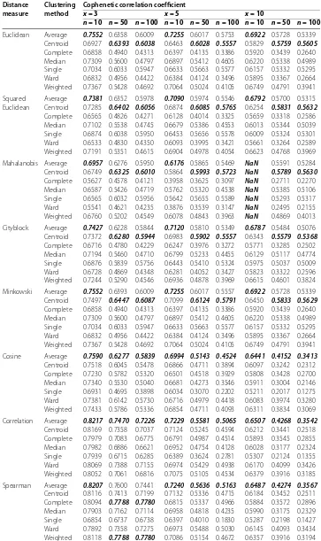
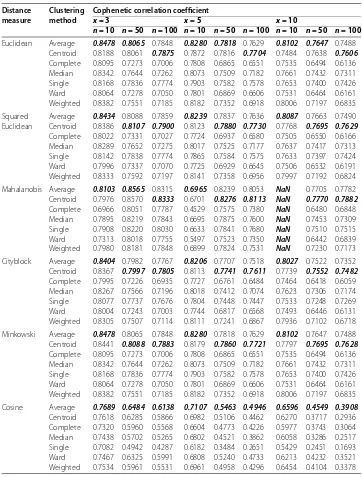
All numerical results, obtained by running the simulation program, are given in Table  and Table . According to Table  and Table , the average method gives the best results at all measures and at all variable numbers for both distributions with sample sizen= . Moreover, increasing the sample size ton=  andn=  favors the complete, weighted, and centroid methods for all measures. However, the cophenetic correlation coeﬃcient for the Mahalanobis measure cannot be calculated in both distributions when there are  variables with sample sizen= , whereas there is not any meaningful explanation for this unexpected result, we still could not ﬁnd the main reason for this situation, but the same result is obtained for more than three times run of the simulation program.

4 Conclusion

(5)

[image:5.595.115.478.108.719.2]

Table 1 The cophenetic correlation coefﬁcient values forμ= 0,σ2_{= 1 (without outliers)}

Distance measure

Clustering method

Cophenetic correlation coefﬁcient

x= 3 x= 5 x= 10

n= 10 n= 50 n= 100 n= 10 n= 50 n= 100 n= 10 n= 50 n= 100

Euclidean Average 0.7552 0.6358 0.6009 0.7255 0.6017 0.5753 0.6922 0.5728 0.5339 Centroid 0.6927 0.6393 0.6038 0.6463 0.6028 0.5557 0.5829 0.5759 0.5605

Complete 0.6858 0.4940 0.4313 0.6397 0.4135 0.3386 0.5920 0.3439 0.2640 Median 0.7309 0.5600 0.4797 0.6897 0.5412 0.4605 0.6220 0.5338 0.4989 Single 0.7034 0.6033 0.5947 0.6633 0.5663 0.5577 0.6157 0.5332 0.5295 Ward 0.6832 0.4956 0.4422 0.6384 0.4124 0.3496 0.5895 0.3367 0.2664 Weighted 0.7367 0.5428 0.4692 0.7064 0.5024 0.4105 0.6749 0.4791 0.3941

Squared Euclidean

Average 0.7381 0.6352 0.5978 0.7090 0.5974 0.5546 0.6792 0.5700 0.5315 Centroid 0.7285 0.6402 0.6056 0.6874 0.6085 0.5765 0.6254 0.5831 0.5632

Mahalanobis Average 0.6957 0.6276 0.5950 0.6176 0.5865 0.5469 NaN 0.5591 0.5284 Centroid 0.6749 0.6325 0.6010 0.5864 0.5993 0.5723 NaN 0.5789 0.5630

Complete 0.5627 0.4578 0.4121 0.3958 0.3625 0.3097 NaN 0.2711 0.2270 Median 0.6587 0.5426 0.4719 0.5762 0.5320 0.4538 NaN 0.5385 0.5106 Single 0.6565 0.6032 0.5956 0.5642 0.5655 0.5589 NaN 0.5293 0.5317 Ward 0.5541 0.4621 0.4235 0.3876 0.3539 0.3147 NaN 0.2495 0.2155 Weighted 0.6760 0.5202 0.4549 0.6078 0.4843 0.3963 NaN 0.4869 0.4013

Cityblock Average 0.7427 0.6228 0.5844 0.7120 0.5810 0.5349 0.6787 0.5484 0.5076 Centroid 0.7372 0.6280 0.5944 0.6983 0.5902 0.5557 0.6343 0.5579 0.5368

Minkowski Average 0.7552 0.6393 0.6009 0.7255 0.6017 0.5557 0.6922 0.5728 0.5339 Centroid 0.7497 0.6447 0.6087 0.7099 0.6124 0.5791 0.6450 0.5833 0.5629

Cosine Average 0.7590 0.6277 0.5839 0.6994 0.5143 0.4524 0.6441 0.4152 0.3413

Centroid 0.7518 0.6045 0.5478 0.6866 0.4711 0.3894 0.6097 0.3242 0.2312 Complete 0.7230 0.5782 0.5320 0.6501 0.4518 0.3929 0.5808 0.3428 0.2700 Median 0.7340 0.5530 0.5040 0.6681 0.4273 0.3546 0.5911 0.3004 0.2146 Single 0.6931 0.4695 0.3898 0.6034 0.3070 0.2202 0.5211 0.2017 0.1275 Ward 0.7381 0.6142 0.5730 0.6716 0.4979 0.4418 0.6083 0.3974 0.3280 Weighted 0.7433 0.5786 0.5336 0.6854 0.4711 0.4093 0.6311 0.3834 0.3069

Correlation Average 0.8217 0.7470 0.7226 0.7229 0.5581 0.5065 0.6507 0.4268 0.3542

Spearman Average 0.8207 0.7600 0.7441 0.7240 0.5636 0.5163 0.6487 0.4274 0.3567

(6)

Table 1 (Continued)

x= 3 x= 5 x= 10

n= 10 n= 50 n= 100 n= 10 n= 50 n= 100 n= 10 n= 50 n= 100

Chebychev Average 0.7375 0.6183 0.5804 0.6933 0.5595 0.5141 0.6448 0.4958 0.4523 Centroid 0.7317 0.6241 0.5870 0.6811 0.5693 0.5334 0.6100 0.5067 0.4805

[image:6.595.117.479.95.205.2]

Table 2 The cophenetic correlation coefﬁcient values forμ= 0,σ2_{= 1 (with outliers)}

x= 3 x= 5 x= 10

n= 10 n= 50 n= 100 n= 10 n= 50 n= 100 n= 10 n= 50 n= 100

Euclidean Average 0.8478 0.8065 0.7848 0.8280 0.7818 0.7629 0.8102 0.7647 0.7488 Centroid 0.8188 0.8061 0.7875 0.7872 0.7816 0.7704 0.7484 0.7638 0.7606

Squared Euclidean

Average 0.8434 0.8088 0.7859 0.8239 0.7837 0.7636 0.8087 0.7663 0.7490 Centroid 0.8386 0.8107 0.7900 0.8123 0.7880 0.7730 0.7768 0.7695 0.7629

Mahalanobis Average 0.8103 0.8565 0.8315 0.6965 0.8239 0.8053 NaN 0.7705 0.7782 Centroid 0.7976 0.8570 0.8333 0.6701 0.8276 0.8113 NaN 0.7770 0.7882

Complete 0.6966 0.8051 0.7787 0.4529 0.7575 0.7380 NaN 0.6480 0.6848 Median 0.7895 0.8219 0.7843 0.6695 0.7875 0.7600 NaN 0.7453 0.7309 Single 0.7908 0.8220 0.8030 0.6633 0.7841 0.7680 NaN 0.7510 0.7515 Ward 0.7313 0.8018 0.7755 0.5497 0.7523 0.7350 NaN 0.6442 0.6839 Weighted 0.7980 0.8181 0.7848 0.6899 0.7824 0.7531 NaN 0.7230 0.7173

Cityblock Average 0.8404 0.7982 0.7767 0.8206 0.7707 0.7518 0.8027 0.7522 0.7352 Centroid 0.8367 0.7997 0.7805 0.8113 0.7741 0.7611 0.7739 0.7552 0.7482

Minkowski Average 0.8478 0.8065 0.7848 0.8280 0.7818 0.7629 0.8102 0.7647 0.7488 Centroid 0.8441 0.8088 0.7883 0.8179 0.7860 0.7721 0.7797 0.7695 0.7628

Cosine Average 0.7689 0.6484 0.6138 0.7107 0.5463 0.4946 0.6596 0.4549 0.3908

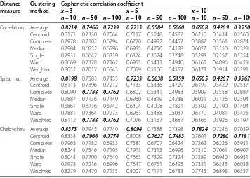
[image:6.595.116.478.257.734.2]

(7)

Table 2 (Continued)

x= 3 x= 5 x= 10

n= 10 n= 50 n= 100 n= 10 n= 50 n= 100 n= 10 n= 50 n= 100

Correlation Average 0.8214 0.7466 0.7239 0.7213 0.5584 0.5060 0.6508 0.4269 0.3550

Spearman Average 0.8198 0.7583 0.7455 0.7233 0.5638 0.5159 0.6505 0.4267 0.3567

Centroid 0.8113 0.7396 0.7212 0.7133 0.5336 0.4729 0.6199 0.3429 0.2537 Complete 0.8090 0.7788 0.7762 0.6802 0.5341 0.4983 0.5909 0.3558 0.2887 Median 0.7887 0.7136 0.7140 0.6960 0.4819 0.4238 0.6021 0.3126 0.2304 Single 0.6861 0.6736 0.6742 0.6404 0.4008 0.1821 0.5302 0.2190 0.1404 Ward 0.7881 0.7364 0.7273 0.6963 0.5488 0.5037 0.6170 0.4081 0.3425 Weighted 0.8112 0.7788 0.7762 0.7076 0.5157 0.4687 0.6366 0.3926 0.3197

Chebychev Average 0.8373 0.7945 0.7740 0.8094 0.7588 0.7398 0.7824 0.7246 0.7059 Centroid 0.8338 0.7966 0.7774 0.8008 0.7627 0.7483 0.7601 0.7280 0.7181

One may conclude that the results of this study, which is similar to ﬁndings of Johnson and Wichern [], indicate the data set with outliers have higher cophenetic correlation values than the data set without outliers.

This study hopes to contribute to literature for making better decisions on selection of appropriate cluster methods by using subgroup sizes, variable numbers, subgroup means and variances.

Competing interests

The authors declare that they have no competing interests.

Authors’ contributions

SS has made intellectual contributions in order to carry out this study and also has carried out the simulation study. ND has determined the research design as well as has coordinated the whole process. ˙ID has made theoretical contributions and has performed statistical analysis of the study. All authors read and approved the ﬁnal manuscript.

Author details

1_{Department of Statistics, Faculty of Arts and Sciences, Afyon Kocatepe University, Afyonkarahisar, 03200, Turkey.} 2_{Department of Biostatistics, Faculty of Medicine, Afyon Kocatepe University, Afyonkarahisar, 03200, Turkey.}

Acknowledgements

Dedicated to Professor Hari M Srivastava.

The authors would like to thank Rıdvan ÜNAL for support of technical help. He is a lecturer at the Afyon Kocatepe University, Faculty of Science, Department of Physics, Afyonkarahisar/Turkey.

Received: 31 December 2012 Accepted: 10 April 2013 Published: 23 April 2013

References

1. Carmichael, JW, George, JA, Julius, RS: Finding natural clusters. Syst. Zool.17(2), 144-150 (1968)

2. Lapointe, FJ, Legendre, P: Comparison tests for dendrograms: a comparative evaluation. J. Classif.12, 265-282 (1995) 3. Kettenring, JR: The practice of cluster analysis. J. Classif.23, 3-30 (2006)

4. Gunnarsson, J: Portfolio-Based Segmentation and Consumer Behaviour: Empirical Evidence and Methodological Issues. Ph.D. Dissertation, Stockholm School of Economics, The Economic Research Institute, p. 274 (1999) 5. Steinbach, M, Karypis, G, Kumar, V: A comparison of document clustering techniques. Text mining workshop. In: Proc.

of the Sixth ACM SIGKDD International Conference on Knowledge Discovery and Data Mining (KDD 2000), Boston, MA, pp. 20-23 (2000)

[image:7.595.118.474.97.351.2]

(8)

7. Lessig, VP: Comparing cluster analyses with cophenetic correlation. J. Mark. Res.9(1), 82-84 (1972)

8. Sneath, HA, Sokal, RR: Numerical Taxonomy: The Principles and Practice of Numerical Classiﬁcation, p. 573. Freeman, San Francisco (1973)

9. Mathworks statistics toolbox: http://www.mathworks.com/help/stats/cophenet.html (2012) 10. Sokal, RR, Rohlf, FJ: The comparison of dendrograms by objective methods. Taxon11, 33-40 (1962) 11. Farris, JS: On the cophenetic correlation coeﬃcient. Syst. Zool.18(3), 279-285 (1969)

12. Rohlf, FJ, David, LF: Test for hierarchical structure in random data sets. Syst. Zool.17, 407-412 (1968)

13. Baker, FB: Stability of two hierarchical grouping techniques - case I: sensitivity to data errors. J. Am. Stat. Assoc.69, 440-445 (1974)

14. Hubert, L: Approximate evaluation techniques for the single-link and complete-link hierarchical clustering procedures. J. Am. Stat. Assoc.69, 698-704 (1974)

15. Kuiper, FK, Fisher, LA: A Monte Carlo comparison of six clustering procedures. Biometrics31, 777-783 (1975) 16. Blashﬁeld, RK: Mixture model tests of cluster analysis: accuracy of four agglomerative hierarchical methods. Psychol.

Bull.83, 377-388 (1976)

17. Milligan, GW: An examination of the eﬀect of six types of error perturbation on ﬁfteen clustering algorithms. Psychometrika45, 325-342 (1980)

18. Hands, S, Everitt, B: A Monte Carlo study of the recovery of cluster structure in binary data by hierarchical clustering techniques. Multivar. Behav. Res.22, 235-243 (1987)

19. Yao, KB: A comparison of clustering methods for unsupervised anomaly detection in network traﬃc. Ph.D. Thesis, University of Copenhagen (2006)

20. Ferreira, L, Hitchcock, DB: A comparison of hierarchical methods for clustering functional data. Commun. Stat., Simul. Comput.,38, 1925-1949 (2009)

21. Milligan, GW, Cooper, MC: A study of standardization of variables in cluster analysis. J. Classif.5, 181-204 (1988) 22. Dixon, WJ: Analysis of extreme value. Ann. Math. Stat.21, 488-506 (1950)

23. Johnson, RA, Wichern, DW: Applied Multivariate Statistical Analysis, 5th edn. Prentice Hall, New York (2002)

doi:10.1186/1029-242X-2013-203

Cite this article as:Saraçli et al.:Comparison of hierarchical cluster analysis methods by cophenetic correlation.