R E S E A R C H
Open Access
Estimation in a partially linear single-index
model with missing response variables
and error-prone covariates
Xin Qi
1,2and De-Hui Wang
1**Correspondence: [email protected] 1College of Mathematics, Jilin University, Changchun, 130012, P.R. China
Full list of author information is available at the end of the article
Abstract
In this paper, the authors study the partially linear single-index model when the covariateXis measured with additive error and the response variableYis sometimes missing. Based on the least-squared technique, an imputation method is proposed to estimate the regression coefficients, single-index coefficients, and the nonparametric function, respectively. Thereafter, asymptotical normalities of the corresponding estimators are proved. A simulation experiment and an application to a diabetes study are used to illustrate our proposed method.
Keywords: partially linear single-index model; least-squared; local linear regression; imputation estimator
1 Introduction
We study the partially linear single-index model
Y=gZTα+XTβ+ε, (.)
whereYis a response variable, (Z,X)∈Rp×Rqis covariate,g(·) is an unknown univari-ate measurable function,ε is a random error withE(ε|Z,X) = ,Var(ε|Z,X) =σ<∞, and (α,β) is an unknown vector inRp×Rqwithα= . The restrictionα= ensures identifiability.
In recent years, model (.) has attracted broad attention because it includes two impor-tant semi-parametric models as its special cases: the single model (Ichimura []) and the partially linear model (Engleet al.[]). Relevant studies about model (.) have been done by Carrollet al.[], Yuet al.[], Lianget al.[], Xiaet al.[] and Xueet al.[], all of which based on the complete data set.
In practice, missing-data problems are always caused by design or accident, so the statis-ticians, such as Liuet al.[] and Laiet al.[], have paid a great attention to them. Most of these researches concerning missing-data problems have been carried out on the con-dition that the covariates can be observed exactly. However, observations are often mea-sured with errors, as can be seen in the papers of Lianget al.[] and Chenet al.[]. Never-theless, those studies of the observations characterized by inaccurate measures are based on the complete data set. Therefore, it is necessary to study error-in-variables models with
missing response. Taking both measurement errors in the covariates and the missing re-sponse variables into account, Lianget al.[], Weiet al.[] and Wei [] have done some work in the partially linear model, in the partially linear additive model and in the partially linear varying-coefficient model, respectively.
The common method of dealing with missing data is the imputation method which was developed by Wanget al.[] in the partially linear model. This paper, with the enlight-enment of Laiet al.[], focuses on estimatingβ,α, and the nonparametric functiong(·) with imputation method when the covariateXis measured with additive error and the response variableYis sometimes missing in the model (.). It is assumed that the obser-vationVis a substitute ofX
V=X+U. (.)
Theδ= indicates thatY is missing, otherwiseδ= . We assume that the measurement error Uis independent from (Y,Z,X,δ) with E(U) = andcov(U) =uu. At first, it is assumed thatuuis known. If it is unknown, it can be estimated with partial replication (Lianget al.[]). Throughout this paper, we assume the data missing mechanism is as follows:
p(δ= |Y,Z,X) =p(δ= |Z,X) =π(Z,X) (.)
for some unknownπ(Z,X). In addition,p(δ= |Y,Z,X,V) =π(Z,X), this is because the measurement errorUis independent from (Y,Z,X,δ). As is pointed out by Lianget al. [], sinceXis observed with measurement error,Yis therefore not missing at random if no further assumptions are made.
The rest of this paper is organized as follows. In Section , the imputation method is used to estimate the parameters and nonparametric function. In Section , relative asymptotic results are presented. In Section , some simulation is conducted to illustrate the proposed approach, and we apply our method to analyze a diabetes data set. All proofs are shown in Section .
2 Methodology
In the following, let{(Yi,Zi,Xi,Vi,Ui,δi),i= , , . . . ,n}be independent and identically dis-tributed, and writeA⊗=A·AT.
2.1 Complete method
In order to derive the imputation estimators, first we define the complete estimators ofβ,
α, and the nonparametric functiong(·). Note thatδiYi=δig(ZiTα) +δiXTi β+δiεi. Taking conditional expectations givenZTα, from the assumptions, we have
EδiYi|ZTiα
=Eδi|ZiTα
gZTi α+EδiXi|ZiTα
T
β.
By multiplying the both sides of model (.) withE(δi|ZiTα), we obtain
Eδi|ZiTα
Yi=E
δi|ZiTα
gZTi α+Eδi|ZTi α
XiTβ+Eδi|ZTiα
Then making some straightforward calculations, we get
δi
Yi–m
ZiTα=δi
Xi–m
ZiTαTβ+δiεi, (.)
wherem(t) =EE(δ(δX|Z|ZTTαα==tt)),m(t) =
E(δY|ZTα=t)
E(δ|ZTα=t) . Ifm(t),m(t) are known and theXiare ob-served, according to (.), the least-square estimator ofβcan be defined as
ˆ β=
n
n
i=
δi
Xi–m
ZTiα⊗
–
·
n
n
i=
δi
Xi–m
ZTiαYi–m
ZTi α
.
However, theXiare measured with error andm(ZiTα),m(ZTiα) are unknown. From our assumptions, it follows thatE(δV|ZTα) =E(δX|ZTα). Therefore, the estimator ofβby the correction for the attenuation technique can be defined as
ˆ βn=
n
n
i=
δi
Vi–mˆ
ZiTα⊗–uu
–
·
n
n
i=
δi
Vi–mˆ
ZTi αYi–mˆ
ZiTα
, (.)
wheremˆ(ZTi α) andmˆ(ZTiα) are the estimators ofm(ZiTα) andm(ZTi α), respectively,
andm(t) =EE(δ(δV|Z|ZTTαα==t)t). LetKh(t) =
K(ht )
h , withK(·) being a kernel function andhbeing
a suitable bandwidth. Those estimators are defined as
ˆ
m(t) = n
i=
δiKh(ZTiα–t) n
i=δiKh(Z
T i α–t)
Yi, mˆ(t) = n
i=
δiKh(ZTiα–t) n
i=δiKh(Z
T iα–t)
Vi.
After obtaining the estimator ofβ, we try to estimateg(·) andg(·) for any fixedα, based onβˆn. In fact, it becomes a single-index model which isY–XTβ=g(ZTα) +ε. Taking conditional expectations givenZTαon the above formula, from the previous assumptions, there isg(t,α,β) =E(Y–XTβ|ZTα=t) =E(Y –VTβ|ZTα=t). Thus, estimatingg(·) is not necessary to be corrected. By a local linear method, we approximateg(t) within the neighborhood oft,g(t)≈g(t) +g(t)(t–t). Then we can obtain the estimators ofg(·) andg(·) by minimizing
min
g(t),g(t)
n
i=
Yi–ViTβˆn–g(t) –g(t)(ti–t)
Kh(ti–t)δi,
whereKh(t) =
K(ht)
h , withK(·) being a kernel function andhbeing a suitable bandwidth.
Through a direct calculation, we have
ˆ
gn(t)
hgˆn(t)
= n
n
i=
nB
T SB
–
BiδiKh(ti–t)
Yi–ViTβˆn
where
Bi=
ti–t
h
, i= , , . . . ,n, B=
⎛ ⎜ ⎜ ⎝
BT .. . BTn
⎞ ⎟ ⎟ ⎠,
S=
⎛ ⎜ ⎜ ⎝
δKh(t–t)
. ..
δnKh(tn–t)
⎞ ⎟ ⎟ ⎠.
In order to apply the above formulas, we have to know the estimation values ofα, which can be obtained by the following formula:
ˆ αn=min
α
n
i=
δi
Yi–ViTβˆn–gˆn
ZTiα. (.)
The complete estimation procedure consists of the following steps:
Step . Select an initial valueαˆ, for example, using an available method, such as the
com-plete data estimation method proposed by Xiaet al.[], and letαˆn= ˆααˆ.
Step . Based on (.) and (.), we can getβˆnk,gˆnk(·)whenα=αˆn.
Step . The solution of (.) is written asαˆn(k+). Letαˆn= ˆ
αn(k+)
ˆαn(k+). Step . Iterate Steps and until convergence is achieved.
2.2 Imputation method
In this part, we will use the imputation technique to estimateβ,α, and the nonparametric functiong(·). The advantage of this method is that all data can be used. First, we getβˆn,αˆn, andgˆn(·) by the complete method. LetYi◦=δiYi+ ( –δi)[g(ZiTα) +ViTβ], that is,Yi◦=Yi ifδi= ,Yi◦=g(ZTi α) +ViTβ, otherwise. From (.), we haveE(Y◦|Z,X) =g(ZTα) +XTβ. This implies
Yi◦=gZTiα+XiTβ+ei, (.)
whereE(ei|Zi,Xi) = . It is just the form of the partial linear single-index model. Therefore, the least-square estimator ofβcan be defined as
˘ β=
n
n
i=
Xi–E
X|ZTi α⊗
–
·
n
n
i=
Xi–E
X|ZTiαYi◦–EY◦|ZiTα
.
for the attenuation technique, the imputation estimator ofβcan be defined as
˘ βn=
n
n
i=
Vi–Eˆ
V|ZTiα⊗–uu
–
·
n
n
i=
Vi–Eˆ
V|ZiTαYi∗–EˆY∗|ZiTα– n
n
i=
( –δi)uuβˆn
, (.)
whereEˆ(V|ZT
i α),Eˆ(Y∗|ZTiα) are the estimators ofE(V|ZiTα),E(Y∗|ZTiα), respectively. Let
Kh(t) =
K(ht)
h , withK(·) being a kernel function andhbeing a suitable bandwidth. Those
estimators are defined as
ˆ
E(V|t) = n
i=
Kh(Z
T i α–t) n
i=Kh(Z
T iα–t)
Vi, Eˆ
Y∗|t= n
i=
Kh(Z
T iα–t) n
i=Kh(Z
T i α–t)
Yi∗.
Similarly, we obtain the imputation estimators ofg(t) andg(t) by
min
g(t),g(t)
n
i=
Yi∗–ViTβ˘n–g(t) –g(t)(ti–t)
Kh(ti–t), (.)
whereKh(t) =
K(ht )
h , withK(·) being a kernel function andhbeing a suitable
band-width. Through a direct calculation, we have
˘
gn(t) hg˘n(t)
= n
n
i=
nB
T SB
–
BiKh(ti–t)
Yi∗–ViTβ˘n
, (.)
where
Bi=
ti–t
h
, i= , , . . . ,n, B=
⎛ ⎜ ⎜ ⎝
BT .. . BTn
⎞ ⎟ ⎟ ⎠,
S=
⎛ ⎜ ⎜ ⎝
Kh(t–t) . ..
Kh(tn–t)
⎞ ⎟ ⎟ ⎠.
As in the complete situation, if we want to use (.) and (.), it is a must to estimateα
first, by minimizing the sum of square errors
min
α
n
i=
Yi∗–ViTβ˘n–g˘n
ZiTα, (.)
sayα˘n. Next we do the same work as in the complete situation.
3 Asymptotic results
In this section, the main results of this paper are summarized. For a concise representa-tion, letS=S–EE(δ(δS|Z|ZTTαα==tt)) andS=S–E(S|ZTα=t), for example,X=X–
E(δX|ZTα=t)
X–m(t),X=X–E(X|ZTα=t). Moreover, in order to state the asymptotic results, the following assumptions will be used.
(C) The matrix X|Z=E{δ[X–m(t)]⊗}is a positive-definite.
(C) Each entry of the Hessian matrices ofm(t)andm(t)is continuous and squared
in-tegrable, where the(i,j)entry of a Hessian matrix ofg(z)is defined as∂∂zg(z) i∂zj. (C) The bandwidths are of ordern–
p+, wherepis the dimension ofZ.
(C) The kernelsKi(·),i= , , , are a bounded symmetric density functions with
com-pact support[–, ], and they satisfyuKi(u)du= ,
uK
i(u)du= .
(C) The density functionf(t)ofZTαis bounded away from and has two bounded
deriva-tives on its support.
(C) g(·),m(·),m(·),E(V|·),E(Y∗|·)have two bounded, continuous derivatives on their
supports.
(C) The probability functionπ(Z,X)has bounded continuous second partial derivatives,
and is bounded away from zero on the support of(Z,X). (C) E(|ε|<∞),E(|U|<∞).
Now we give the following asymptotical results.
Theorem . Assume that the conditions(C)-(C)are satisfied,then we obtain
√
n(β˘n–β)→N
,–
Xβ∗ –
X
,
whereX=E{X ⊗
},β∗=E[{( X+– –Z ZX) X–·δ(X(ε–U
Tβ) +εU– (UUT–
uu)β) – –Z δZg (ZTα)(ε– UTβ)}⊗], with =E{( –δ)XXT} and =E{( –
δ)X[Zg(ZTα)]T}.
Theorem . Suppose the conditions(C)-(C)are satisfied,then we have
√
n(α˘n–α)→N
,–
ZXα∗ –
ZX
,
whereZX=E{ZX T
g(t)},α∗=E[(Q+P)⊗],with Q and P given in(.)and(.)of
Section,respectively.
Theorem . Suppose that the conditions(C)-(C)hold,we have
nh
ˇ
gn(t;αˇn,βˇn) –g(t)
→N
,μ(t)γ(K)g f(t)
,
whereγ(K) =
K (u)du.
4 Numerical examples
4.1 Simulation
In this subsection, we carry out some Monte Carlo experiments to show the finite sample performance of the proposed method. The set of data is generated from the following model:
Yi=sin
Table 1 Biases ofαandβunder different missing functions and different sample sizes obtained by two different methods for the simulated data
Complete Imputation
Missing rate n α1ˆ α2ˆ α3ˆ βˆ α1˘ α2˘ α3˘ β˘
0.30 50 0.0035 0.0041 –0.0057 0.0308 –0.0026 0.0037 –0.0031 0.0172
100 0.0032 –0.0018 –0.0024 0.0230 0.0016 –0.0009 –0.0010 0.0092 150 0.0036 –0.0012 –0.0026 0.0234 0.0016 –0.0005 –0.0011 0.0093
0.20 50 0.0033 0.0023 –0.0047 0.0206 –0.0012 0.0009 –0.0008 0.0147
100 0.0030 –0.0018 –0.0023 0.0162 0.0012 –0.0007 –0.0005 0.0089 150 0.0031 –0.0011 –0.0024 0.0167 0.0013 –0.0003 –0.0006 0.0091
0.10 50 0.0021 0.0009 –0.0029 0.0132 –0.0005 0.0005 0.0004 0.0101
100 0.0022 –0.0009 –0.0013 0.0097 0.0003 –0.0002 –0.0004 0.0063 150 0.0022 –0.0009 –0.0015 0.0096 0.0004 –0.0002 –0.0005 0.0056
Table 2 Standard errors ofαandβunder different missing functions and different sample sizes obtained by two different methods for the simulated data
Complete Imputation
Missing rate n α1ˆ α2ˆ α3ˆ βˆ α1˘ α2˘ α3˘ β˘
0.30 50 0.1011 0.0883 0.0969 0.1108 0.0694 0.0586 0.0684 0.0778
100 0.0470 0.0467 0.0471 0.0662 0.0282 0.0288 0.0288 0.0448 150 0.0333 0.0331 0.0334 0.0512 0.0212 0.0215 0.0214 0.0348
0.20 50 0.0813 0.0782 0.0845 0.0995 0.0433 0.0416 0.0429 0.0626
100 0.0438 0.0438 0.0443 0.0601 0.0242 0.0247 0.0251 0.0369 150 0.0315 0.0315 0.0313 0.0475 0.0184 0.0191 0.0186 0.0291
0.10 50 0.0711 0.0731 0.0753 0.0937 0.0345 0.0327 0.0345 0.0515
100 0.0405 0.0399 0.0412 0.0560 0.0200 0.0204 0.0210 0.0306 150 0.0293 0.0290 0.0292 0.0441 0.0155 0.0159 0.0156 0.0239
where α = √ (, , )
T, β= , X
i∼N(, ),εi∼N(, .),Ui∼N(, .), the Zi are trivariate with independentU(, ) components. Throughout this section, the kernel func-tionKi(t) =( –t)if|t| ≤ (i= , , , ) is used. Thehi(i= , , , ) are taken as the related bandwidths.
Based on this model, we considered the following three data missing mechanisms of the response, respectively:
Case . P(δ= |Z=z,X=x) = . + .(|zTα– .|+|x– |)if|zTα– .|+|x– | ≤, and
. elsewhere;
Case . P(δ= |Z=z,X=x) = . – .(|zTα– .|+|x– |)if|zTα– .|+|x– | ≤, and
. elsewhere;
Case . P(δ= |Z=z,X=x) = .for allzandx.
The average missing rates are ., ., and ., respectively. For each case, we gen-erated random samples of sizen= , , , respectively. The estimators with standard error (SE) ofαandβunder different missing mechanisms, obtained by two dif-ferent methods for the simulated data, are reported in Tables and . The relative mean integrated square error (MISE) ofg(·) under different missing mechanisms, obtained by two different methods for the simulated data, is reported in Table .
[image:7.595.117.478.279.408.2]Table 3 The relative mean integrated square error ofg(·) under different missing functions and different sample sizes obtained by two different methods for the simulated data
Complete Imputation
Missing rate n gˆn(·) g˘n(·)
0.30 50 0.2014 0.1227
100 0.1251 0.0921
150 0.1014 0.0915
0.20 50 0.1514 0.0930
100 0.1102 0.0915
150 0.1026 0.0918
0.10 50 0.1451 0.0923
100 0.1138 0.0910
150 0.0996 0.0906
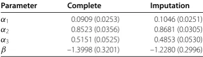
Table 4 The estimates and standard errors ofαandβby two different methods from the diabetes data
Parameter Complete Imputation
α1 0.0909 (0.0253) 0.1046 (0.0251)
α2 0.8523 (0.0356) 0.8681 (0.0305)
α3 0.5151 (0.0525) 0.4853 (0.0530)
β –1.3998 (0.3201) –1.2280 (0.2996)
As the sample size increases, the bias and SE of these estimators decrease for any fixed missing rate. Furthermore, as the missing rate decreases, the bias and SE of these estima-tors decrease for any fixed sample size. From Table , the imputation estimatorg˘(·) has a better performance than the complete estimatorgˆ(·) in terms of MISE.
4.2 Application to diabetes data
In this part, we will elaborate on the proposed method through an analysis of data set from a diabetes study. Using partially linear additive model, Gaiet al.[] have analyzed the data set which includes observations for diabetes patients. The response variable Y is employed as a quantitative measurement of disease progression one year after base-line. The covariates include age, body mass index (BMI), average blood pressure (BP) and glucose concentration. In our notation,Z= (age,BMI,BP)T,Xis the glucose concentra-tion measured with error. We have two replicates ofW, the error-prone measurement of the glucose concentration, and we apply them into estimation of the measurement error variance. The precise procedures, containing the modified asymptotic variance forαand
β, are depicted in Section of Lianget al.[]. We carry out a sensitivity analysis by taking
σuu= .. In order to use the data set to demonstrate our methods, we presume that %of theY values are missed.
The estimated values of parameters of interest via using the complete method and im-putation method are presented in Table . It is shown that imim-putation estimators have smaller standard errors than complete estimators.
5 Proofs of the main results
In order to prove the main results, we first give some lemmas.
Lemma . Assume that the conditions(C)-(C)hold,then we have
[image:8.595.197.397.278.334.2]whereϕ(·)defines one of m(·),m(·),m(·),andϕˆ(·)is for the estimators ofϕ(·).
The proof of Lemma . can be finished with the work by Market al.[] and Theo-rems , by Einmahlet al.[].
Lemma . Assume that the conditions(C)-(C)hold,then we have
√
n(βˆn–β)→N
, –Xβ X–
,
where X=E{δX⊗},β=E{δ[(ε–UTβ)X]⊗}+E{δ[(UUT–uu)β]⊗}+E[δ(UUTε)]. The proof of Lemma . is similar to the proof of Theorem by Lianget al.[]. So the details are omitted here.
Lemma . Under the conditions(C)-(C)hold,then we have
√
n(αˆn–α)→N
, Z–α –Z
,
where Z=E{δ[Zg(t)]⊗},α=E{δ{[Zg(t) – ZX –XX](ε–U
Tβ) +
ZX X–[(UU T–
uu)β–Uε]}}⊗,with ZX=E[δZXTg(t)].
The proof of Lemma . uses a similar method to the proof of Theorem . by Liang et al.[]. Here, we only give some key steps. First, we derive the following expression:
ˆ
gn(t,αˆn,βˆn) –g(t)
= n·
f(t)μ(t)
n
i=
δiKh
ZTi α–t
εi–UiTβ
– (βˆn–β)T
E(δX|ZTα=t) E(δ|ZTα=t
)
– (αˆn–α)T
E(δZg(ZTα)|ZTα=t) E(δ|ZTα=t
)
+op
√
n
+Op
h, (.)
whereμ(t) =E(δ|ZTα=t). Then we can obtain
√
n Z(αˆn–α) =
√
n
n
i=
δig
ZTiαZi
εi–UiTβ
–√n ZX(βˆn–β) +op().
Combining Lemma . and the central limit theorem, we can complete the proof of Lemma ..
Lemma . Suppose that the conditions(C)-(C)hold,we have
nh
ˆ
gn(t;αˆn,βˆn) –g(t) – μ(K)g
(t)h
→N
,γ(K)g f(t)
,
whereμ(K) =uK(u)du,γ(K) =K
Proof Note thatαˆn–α=Op(n–
), sogˆn(t;αˆn,βˆn) –gˆn(t;α,βˆn) =Op(n–). Then we only
need to obtain the asymptotic expansion ofgˆn(t;α,βˆn). From (.), we have
ˆ
gn(t;α,βˆn)
hgˆn(t;α,βˆn)
–
g(t) hg(t)
=
nB
T SB
– n
n
i=
BiδiKh(ti–t)
×
ti–t h
g(t)h+εi–UiTβ
–ViT(βˆn–β) +op
h. (.)
As is pointed out by Laiet al.[],
nB
T
SB=μ(t)f(t)
μ(K)
+op()
, (.)
n
n
i=
BiδiKh(ti–t)
ti–t h
g(t)h
=
f(t)μ(t)μ(K)g(t)h
+op
√
nh
. (.)
Combine (.), (.), and (.) and focus on the top equation, it follows that
ˆ
gn(t;α,βˆn) –g(t)
= μ(K)g
(t)h
+ n
n
i=
μ(t)f(t)δiKh(ti–t)
εi–UiTβ
–ViT(βˆn–β)
+op
√
nh
.
Because of Lemma ., it is easy to obtain
n
n
i=
μ(t)f(t)δiKh(ti–t)V
T
i (βˆn–β) =op
√
nh
,
then we know that
ˆ
gn(t;αˆn,βˆn) –g(t) = μ(K)g
(t)h
+ n
n
i=
μ(t)f(t)
δiKh(ti–t)
εi–UiTβ
+op
√
nh
.
Applying the central limit theorem, we obtain Lemma ..
Proof of Theorem. Let
n= n
n
i=
Vi–Eˆ
V|ZTiα⊗–uu
Then
n=E
X–EX|ZTα⊗+op() =EX ⊗
+op() =X+op().
By Lemmas .-., it is easy to show that
√
n(βˇn–β) =–n
√ n n i=
ViY∗i–Vi T
β
+–n
√
nuuβ– √ n n i=
( –δi)uuβˆn
+op().
Because of the Taylor expansion and the continuity ofg(·), we obtain
ˆ
gn
ZTi αˆn
–gZTi α
=gˆn
ZiTα+gZTi αZTiαˆn–ZTiα
–gZTi α+op
√ n . (.)
Note thatE(Y∗|ZT
iα) =g(ZTiα) +E(X|ZTi α)Tβ. Using (.) yields
Y∗ i–Vi
T
β= ( –δi)
ˆ gn ZT iα
–gZT i α
+ ( –δi)g
ZT iα
ZT i (αˆn–α)
+ ( –δi)ViT(βˆn–β) +δi
εi–UiTβ
+op
√ n . (.)
Combining (.) and (.), and calculating directly, we have
√
n(βˇn–β) =–n
√ n n i=
Viδi
εi–UiTβ
+– n √ n n i=
Vi( –δi)ViT(βˆn–β)
+–n
√ n n i=
Vi( –δi)Zig
ZTiαT(αˆn–α)
+–n
√
nuuβ– √ n n i=
( –δi)uuβˆn
+op()
=–n(I+I+I+I) +op().
By a straightforward calculation,
I= √ n n i=
Xiδi
εi–UiTβ
+δi
εiUi–UiUiTβ
+op(). (.)
From Lemma . and the law of large numbers, it follows that
I= √ n n i=
Xi( –δi)XiT(βˆn–β) + √ n n i=
=√n· –X · n
n
i=
δiXi
εi–UiTβ
+Uiεi–
UiUiT–uu
β
+√ n
n
i=
( –δi)uu(βˆn–β) +op()
=I+I+op(), (.)
where
=E
( –δ)XXT. (.)
Using Lemma .,Iis decomposed as
I=
√
n
n
i=
Xi( –δi)Zig
ZTiαT(αˆn–α)
+√ n
n
i=
Ui( –δi)Zig
ZiTαT(αˆn–α) +op()
=√n· –Z · n
n
i=
δiZig
ZiTαεi–UiTβ
–√n· Z– ZX –X
·
n
n
i=
δiXi
εi–UiTβ
+Uiεi–
UiUiT–uu
β+op()
=I–I+op(), (.)
where
=E
( –δ)XZgZTαT. (.)
Also we have
I=
√
n
n
n
i=
δiuuβ– n
n
i=
( –δi)uu(βˆn–β)
. (.)
Combining (.), (.), and (.), we get
I+I+I
=√n
n
n
i=
δiXi
εi–UiTβ
+εiUi–
UiUiT–uu
β
=√n
n
n
i=
δiXi
εi–UiTβ
+εiUi–
UiUiT–uu
β
+op()
=√n X(βˆn–β) +op().
Similarly, we obtain
I–I=
– Z– ZX
–
X ·
√
To sum up,
√
n(βˇn–β) =–n
X+– Z– ZX
–
X
·√n
n n i=
δiXi
εi–UiTβ
+εiUi–
UiUiT–uu
β
––n Z–·
√ n n n i=
δig
ZTiαZi
εi–UiTβ
+op(). (.)
Via the central limit theorem, Theorem . can be proved.
Proof of Theorem. We derive the following expression first:
˘
gn(t,α˘n,β˘n) –g(t)
= n
n
i=δiKh(ZTiα–t)(εi–UiTβ)
n n i=Kh(Z
T iα–t)
+ (βˆn–β)TE
( –δ)X|ZTα=t
+gˆn(t) –g(t)
· –Eδ|ZTα=t
– (β˘n–β)TE
X|ZTα=t
– (α˘n–α)TE
ZgZTα|ZTα=t
+op
√
n
+Op
h. (.)
Based on (.), we have
= n
n
i= Kh
ZiTα˘n–t
ZT
iα˘n–t
·Yi∗–ViTβ˘n–g˘n(t) –g˘n(t)
ZTi α˘n–t
.
Taking only the top equation into account, using a Taylor expansion, and calculating di-rectly, we obtain
n
n
i= Kh
ZiTα–t
˘
gn(t) –g(t)
= n n i= Kh
ZTiα–t
( –δi)ViT(βˆn–β) + ( –δi)
ˆ
gn
ZiTα–gZiTα
+δi
εi–UiTβ
– (β˘n–β)T n
n
i= Kh
ZTiα–t
Vi
– (α˘n–α)T n
n
i= Kh
ZiTα–t
Zig(t) +op
√
n
+Op
h. (.)
Dividing all terms in (.) by n ni=Kh(ZTiα–t), we have
˘
gn(t) –g(t) = n
n
i=δiKh(Z
T
iα–t)(εi–UiTβ)
n n
i=Kh(ZiTα–t)
+ (βˆn–β)T n
n
i=( –δi)Kh(ZiTα–t)Vi
n n
+gˆn(t) –g(t)
n
n
i=( –δi)Kh(Z
T i α–t)
n n
i=Kh(ZiTα–t)
– (β˘n–β)T n
n
i=Kh(ZiTα–t)Vi
n n i=Kh(Z
T i α–t)
– (α˘n–α)T n
n
i=Kh(ZTi α–t)Zig(t)
n n i=Kh(Z
T i α–t)
+op
√
n
+Op
h.
Note that
n
n
i=( –δi)Kh(Z
T
iα–t)Vi
n n
i=Kh(ZiTα–t)
=E( –δ)X|ZTα=t
+op()
,
n
n
i=( –δi)Kh(ZTiα–t)
n n
i=Kh(ZiTα–t)
= –Eδ|ZTα=t
+op()
,
n
n
i=Kh(ZiTα–t)Vi
n n i=Kh(Z
T i α–t)
=EX|ZTα=t
+op()
, and n n i=Kh(Z
T
i α–t)Zig(t)
n n
i=Kh(ZiTα–t)
=EZgZTα|ZTα=t
+op()
.
Thus, equation (.) follows.
Second, we give the proof of Theorem .. From (.),α˘nis the solution of
n n i=
Yi∗–ViTβ˘n–g˘n
ZiTα˘n
· ˘gnZTiα˘n
Zi= ,
it can be rewritten as
n
n
i=
gZiTαZi
Yi∗–ViTβ–gZTiα–g˘n
ZTi α˘n
–gZTi α
–ViT(β˘n–β)
· +op()
= . (.)
Because of the Taylor expansion and the continuity ofg(·), we can obtain
˘
gn
ZTi α˘n
–gZTi α
=g˘n
ZiTα+gZTi αZTiα˘n–ZTiα
–gZTi α+op
√ n . (.)
By (.), (.) can be written as
n
n
i=
gZiTαZi
δi
εi–UiTβ
+ ( –δi)ViT(βˆn–β)
+ ( –δi)
ˆ
gn
ZiTα–gZiTα–g˘n
ZTiα–gZTiα–ViT(β˘n–β) –gZiTαZTi (α˘n–α)
+op()
Applying (.) to the equation, it is easy to obtain √ n n i=
δig
ZTiαZi
εi–UiTβ
–√ n n i=
gZTiαZi· n
n
j=δjKh(ZjTα–ZTi α)(εj–UjTβ)
n n j=Kh(Z
T
j α–ZTiα)
–√ n
n
i=
gZTiαZi
ˆ
gn
ZTiα–gZTiα·δi–E
δ|ZTα=ZTiα
+ (βˆn–β)T √ n n i=
gZTiαZi
( –δi)Vi–E
( –δ)V|ZTα=ZTi α
=√ n
n
i=
gZiTαZi
Zig(ZTi α)
Xi+Ui
T
˘ αn–α
˘ βn–β
+op(). (.)
Note that the second term of the left-hand side of (.) is
√ n n i= δi
εi–UiTβ
EZgZTα|ZTα=ZiTα+op().
Then the first two terms of the left-hand side of (.) are as follows:
√ n n i=
δig
ZTiαZi
εi–UiTβ
–√ n n i= δi
εi–UiTβ
EZgZTα|ZTα=ZiTα
=√ n n i= δi
εi–UiTβZig
ZTiα. (.)
Applying (.) to the third term of the left-hand side of (.), it follows that
√ n n i=
gZTiαZi
δi–E
δ|ZTα=ZiTα·gˆn
ZTiα–gZTi α
=√ n
n
i=
gZiTαZi
δi–E
δ|ZTα=ZTiα
·
n
f(ZT
iα)μ(ZTi α) n
j=
δjKh
ZjTα–ZTiαεj–UjTβ
– (βˆn–β)T √ n n i=
gZTiαZi
δi–E
δ|ZTα=ZiTαE(δX|Z
Tα=ZT i α)
E(δ|ZTα=ZT i α)
– (αˆn–α)T √ n n i=
gZTiαZi
δi–E
δ|ZTα=ZTi α
×E(δZg(ZTα)|ZTα=ZiTα)
E(δ|ZTα=ZT i α)
Similar to the second term of the left-hand side of (.),
J=
√
n
n
i=
δi
εi–UiTβ
×
E[δZg(ZTα)|ZT i α]
E(δ|ZT iα)
–E[E(δ|Z
Tα)Zg(ZTα)|ZT i α]
E(δ|ZT i α)
. (.)
Also, we have
J=
√
n(βˆn–β)TE
δ–Eδ|ZTαE(δX|Z
Tα)
E(δ|ZTα) g
ZTαZ
+op(). (.)
Combining with Lemma ., we have
J=
–
Z
√
n
n
i=
δig
ZTiαZi
εi–UiTβ
–√n ZX(βˆn–β)
T
·Eδ–Eδ|ZTαE[δZg
(ZTα)|ZTα]
E(δ|ZTα) g
ZTαZ
+op(). (.)
The last term of the left-hand side of (.) is
√
n(βˆn–β)TE
( –δ)X–E( –δ)X|ZTαgZTαZ+op(). (.)
Through a direct calculation, the first term of the right-hand side of (.) is
√
nZ(α˘n–α) +op(), (.)
where
Z=EZg
ZTα⊗. (.)
The last term of the right-hand side of (.) is
√
nZX(β˘n–β) +op(), (.)
where
ZX=EZg
ZTαXT. (.)
Combining (.)-(.), and (.), and using Theorem ., (.) becomes
√
nZ(α˘n–α) =
√
n
n
i=
δi
εi–UiTβ
gZT iαZi
–√ n
n
i=
δi
εi–UiTβ
gZTαE[(δ–E(δ|Z
Tα))Z|ZT i α]
+√n(βˆn–β)TE
δ–Eδ|ZTαE(δX|Z
Tα)
E(δ|ZTα) g
ZTαZ
+Eδ–Eδ|ZTαE[δZg
(ZTα)|ZTα]
E(δ|ZTα) g
ZTαZ
T
·
–
Z
√
n
n
i=
δig
ZTiαZi
εi–UiTβ
–Eδ–Eδ|ZTαE[δZg(ZTα)|ZTα]
E(δ|ZTα) g
ZTαZ
T
· –
Z
√
n ZX(βˆn–β)
+√n(βˆn–β)TE
( –δ)X–E( –δ)X|ZTαZgZTα
–ZX –
X
X+– –Z ZX
√
n(βˆn–β)
+ZX –
X –
Z ·
√
n n
n
i=
δig
ZiTαZi
εi–UiTβ
+op()
=F–F+F+F–F+F–F+F+op(). (.)
Through a direct calculation,
Q=F–F+F+F
=
+Eδ–Eδ|ZTαE[δZg
(ZTα)|ZTα]
E(δ|ZTα) g
ZTαZ
T –
Z
+ZX –
X –
Z
·√
n
n
i=
δig
ZiTαZi
εi–UiTβ
. (.)
Combining with Lemma ., we have
P=F–F+F–F
=
Eδ–Eδ|ZTαE(δX|Z
Tα)
E(δ|ZTα) g
ZTαZ
T
–Eδ–Eδ|ZTαE[δZg
(ZTα)|ZTα]
E(δ|ZTα) g
ZTαZ
T –
Z ZX
+E( –δ)X–E( –δ)X|ZTαZgZTαT
–ZX –
X
X+– Z– ZX
–
X
·√
n
n
i=
δiXi
εi–UiTβ
+Uiεi–
UiUiT–uu
β+op(). (.)
Then, with the application of the central limit theorem, Theorem . follows
immedi-ately.
From (.), we have
ˇ
gn(t;α,βˇn)
hgˇn(t;α,βˇn)
–
g(t) hg(t)
=
nB
T SB
– n
n
i=
BiKh(ti–t)
×
( –δi)(βˆn–β)TVi+ ( –δi)
ˆ
gn
ZTi αˆn
–gZTi α
+
ti–t h
g(t)h+δi
εi–UiTβ
– (βˇn–β)TVi
+op
√
nh
. (.)
Byh
h →,n→ ∞, with Lemmas .-., focusing on the top equation, we get
ˇ
gn(t;α,βˇn) –g(t) = n
n
i=
f(t)δiKh(ti–t)
εi–UiTβ
+op
√
nh
.
Applying the central limit theorem, we complete the proof of Theorem ..
Competing interests
The authors declare that they have no competing interests.
Authors’ contributions
The authors contributed equally to the writing of this paper. All authors read and approved the final manuscript.
Author details
1College of Mathematics, Jilin University, Changchun, 130012, P.R. China.2Zhuhai College of Jilin University, Zhuhai, 519000, P.R. China.
Acknowledgements
The authors thank the two referees for carefully reading the paper and for their valuable suggestions and comments, which greatly improved the paper. This work is supported by National Natural Science Foundation of China (Nos. 11271155, 11371168, 11001105, 11071126, 11071269, 11501241), Science and Technology Research Program of Education Department in Jilin Province for the 12th Five-Year Plan (440020031139) and Jilin Province Natural Science Foundation (20130101066JC, 20130522102JH, 20150520053JH, 20101596).
Received: 28 September 2015 Accepted: 9 December 2015 References
1. Ichimura, H: Estimation of single index models. Ph.D. dissertation, Department of Economics, MIT (1987) 2. Engle, RF, Granger, CWJ, Rice, J, Weiss, A: Semiparametric estimates of the relation between weather and electricity
sales. J. Am. Stat. Assoc.81, 310-320 (1986)
3. Carroll, RJ, Fan, JQ, Gijbels, I, Wand, MP: Generalized partially linear single-index models. J. Am. Stat. Assoc.92, 477-489 (1997)
4. Yu, Y, Ruppert, D: Penalized spline estimation for partially linear single-index models. J. Am. Stat. Assoc.97, 1042-1054 (2002)
5. Liang, H, Wang, N: Partially linear single-index measurement error models. Stat. Sin.15, 99-116 (2005)
6. Xia, YC, Härdle, W: Semi-parametric estimation of partially linear single-index models. J. Multivar. Anal.97, 1162-1184 (2006)
7. Xue, L, Zhu, LX: Empirical likelihood confidence regions of the parameters in a partially linear single-index model. J. R. Stat. Soc. B68, 549-570 (2006)
8. Liu, XH, Wang, ZZ, Hu, XM: Estimation in partially linear single-index models with missing covariates. Commun. Stat., Theory Methods41, 3428-3447 (2012)
9. Lai, P, Wang, QH: Semiparametric efficient estimation for partially linear single-index model with responses missing at random. J. Multivar. Anal.128, 33-50 (2014)
10. Chen, X, Cui, HJ: Empirical likelihood for partially linear single-index errors-in-variables model. Commun. Stat., Theory Methods38, 2498-2514 (2009)
11. Liang, H, Wang, SJ, Carrol, RJ: Partially linear models with missing response variables and error-prone covariates. Biometrika94, 185-198 (2007)
13. Wei, CH: Estimation of partially linear varying-coefficient errors-in-variables model with missing responses. Acta Math. Sci.30, 1042-1054 (2010) (in Chinese)
14. Wang, QH, Sun, ZH: Estimation in partially linear models with missing responses at random. J. Multivar. Anal.98, 1470-1497 (2007)
15. Lai, P, Wang, QH: Partially linear single-index model with missing responses at random. J. Stat. Plan. Inference141, 1047-1058 (2011)
16. Liang, H, Härdle, W, Carroll, RJ: Estimation in a semiparametric partially linear errors-in-variables model. Ann. Stat.15, 99-116 (1999)
17. Gai, YJ, Zhang, J, Li, GR, Luo, XC: Statistical inference on partial linear additive models with distortion measurement errors. Stat. Methodol.27, 20-38 (2015)
18. Mark, YP, Silverman, BW: Weak and strong uniform consistency of kernel regression estimates. Z. Wahrscheinlichkeitstheor. Verw. Geb.61, 405-415 (1982)