Vehicle Model Recognition Based on Convolutional Neural Network

2018 International Conference on Information, Electronic and Communication Engineering (IECE 2018) ISBN: 978-1-60595-585-8

Vehicle Model Recognition Based on Convolutional Neural Network

Chao WANG, Yi-yang HUANG*, Bo-wen SHI, Yan-yan HUO,

Xue-bin YANG and Meng-zhu WANG

Beijing Information Science and Technology University, China *Corresponding author

Keywords: Convolutional neural network, Vehicle model recognition.

Abstract. Many types of cars and the large computational quantitylead to the low accuracy and low efficiency for vehicle model recognition,to solve this,a vehicle model recognition method based on convolutional neural network (hereinafter referred to as CNN) is proposed in this paper. The method extracts the feature areas of vehicles by using bounding-box annotations. It randomly adjusts the brightness, contrast and hue of images to reduce the impacts of surrounding environments on the training effects. Finally, N images are randomly selected from the training set for batch training. The network performance comparison and optimization are realized by evaluating parameters such as the number of convolutional layers, learning rate, decay rate, momentum and moving average model. The experimental results show that the method proposed has an accuracy of 70% in recognizing the 10 models of the BMW series.

Introduction

The number of vehicles has increased significantly due to the improvement of people’s living standards, leading to frequent traffic accidents and illegal crimes. Since traditional manual monitoring methods can no longer meet the expectations, there is an urgent need for intelligent traffic administration. Vehicle identification plays an important role in intelligent traffic administration while vehicle model recognition serves as an important direction in the field of vehicle identification. The specific vehicle model is an important feature that is crucial for vehicle-related cases.

Literature [1] established a model that could distinguish between 5 vehicle models by using the vehicle model recognition method based on CNN. However, the neural network was simple in structure and low in accuracy. Based on the front-view images of vehicles, Literature [2] proposed a deep learning-based vehicle model recognition algorithm. It adopted the image preprocessing method for dataset processing, which effectively reduced the impacts of irrelevant factors on network training. In this paper, a high-performance deep CNN model is presented and applied to vehicle model recognition. The network performance comparison and optimization are realized by evaluating parameters such as the number of convolutional layers, learning rate, decay rate, momentum and moving average model. The recognition accuracy reaches 70%.

Convolutional Neural Network

CNN is an important deep learning algorithm that has outstanding performance in the image field. It has made breakthrough progress in the field of image classification, face recognition and object detection in recent years. CNN extracts both high-level and low-level features of images, thereby being referred to as a hierarchical feature learning and classification network.

Structure of CNN

cannot be fulfilled by the neural network if there is no activation function. Finally, loss function is introduced to estimate the inconsistency between the predicted output and the actual output of the neural network. The smaller the loss function is, the better the model robustness will be.

Convolutional Layer. Convolutional layers are responsible for feature extraction. At the convolutional layers, feature maps of the previous layer are convolved with iterative convolutional kernels and put through the activation function to form the output feature map. The formulas are as follows:

 

X=f y

. (1)

y=x*k+b . (2) Where x is the output feature map of the previous layer; k is the convolutional kernel matrix; b is the biasvalue of feature maps of convolutional kernels; y is the feature map obtained by calculating the above formulas; f is the activation function; X, which represents the output feature map of this layer, is obtained by calculating the above formulas.

Pooling Layer. Pooling is an important operation in CNN. It can reduce features while maintaining the local invariance of features. Commonly used pooling operations include maximum pooling, average pooling and random pooling. Wherein, maximum pooling can be expressed as follows:

 

Y=down y . (3) Where y is the output feature map of the previous layer; down is the maximum sampling function. The maximum sampling function is to define the size and step size of partition matrix, divide the feature map into n partition matrices, take the maximum value of each matrix and integrate them into the output feature map Y.

Connection Function of CNN

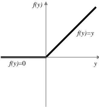
Activation Function. Typical activation functions include ReLU, LeaklyReLU, Parametric ReLU, Randomized ReLU and ELU. Graph and formula of the classic relu function are as follows:

Figure 1. ReLU function.

 

Re

0 0

x ifx

Lu x

ifx  

 _

 . (4)

y f(y)

f(y)=y

Relufunction is a piecewise linear function that turns all negative values into 0 and remains the positive values unchanged. Such unilateral inhibition enables neurons in the neural network to be sparsely activated.

Loss Function. Loss function selection plays an important role in CNN. Representative loss functions include squared error loss, cross entropy loss and hinge loss. Wherein, cross entropy loss can be expressed as follows:





 

 

H p q  



Where p is the expected output; q is the actual output; H(p,q) is the cross entropy.

Network Structure Design

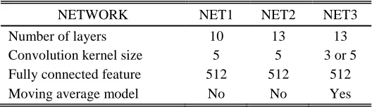
To investigate the impacts of moving average model and number of convolutional layers on the recognition accuracy, a total of three networks are designed in this paper: Network 1, Network 2 and Network 3. Table 1 demonstrates the number of convolutional layers, size of convolutional kernels, feature dimensions of fully-connected layers and moving average models of the three networks.

Table 1. A General Introduction to the Three Networks

NETWORK NET1 NET2 NET3

Number of layers 10 13 13 Convolution kernel size 5 5 3 or 5 Fully connected feature 512 512 512 Moving average model No No Yes

Network 1 consists of 10 layers, including 4 convolutional layers, 4 pooling layers and 2 fully-connected layers. Each convolutional layer is followed by a pooling layer and the last pooling layer is followed by 2 fully-connected layers. In addition, a softmax layer is added for classification. We plan to input color images with the size of 180*200 and extract 6, 12, 24 and 50 feature maps from the 1st, 2nd, 3rd and 4th convolutional layers separately. Finally, 512-dimensional features will be extracted from the fully-connected layers. The size of convolutional kernels in each layer is 5.

Network 2 consists of 13 layers, including 7 convolutional layers, 4 pooling layers and 2 fully-connected layers. Here is a pooling layer after every 2 convolutional layers. The last convolutional layer is followed by a pooling layer while the last pooling layer is followed by 2 fully-connected layers. In addition, a softmax layer is added for classification. We plan to extract 6, 10, 15, 20, 30, 40 and 50 feature maps from the 1st, 2nd, 3rd, 4th, 5th, 6th and 7th convolutional layers separately. Finally, 512-dimensional features will be extracted from the fully-connected layers. The size of convolutional kernels in each layer is 5.

Network 3 consists of 13 layers, including 7 convolutional layers, 4 pooling layers and 2 fully-connected layers. Here is a pooling layer after every 2 convolutional layers. The last convolutional layer is followed by a pooling layer while the last pooling layer is followed by 2 fully-connected layers. In addition, a softmax layer is added for classification. We plan to extract 10, 20, 30, 40, 50, 60 and 70 feature maps from the 1st, 2nd, 3rd, 4th, 5th, 6th and 7th convolutional layers separately, with the convolutional kernel sizes of 5, 3, 5, 5, 3, 3 and 5 respectively. In the meantime, 512-dimensional features will be extracted from the fully-connected layers. Finally, a moving average model will be added to the network. The moving average model can be expressed as follows:





var





var



1-

var

shadow

iable

decay shadow

iable

decay

iable

to control the model update velocity. The moving average model is designed to control the variable update velocity and prevent the impacts of sudden changes in local variables.

Experiment

The experiment was computed on a computer with 2.2 GHz CPU, Intel Core i7 processor and 16GB memory. It was implemented with Anaconda (under MAC), tensor flow machine learning framework and python.

Dataset and Preprocessing

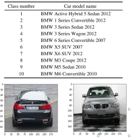
The experimental dataset was provided by Stanford University. It contained a total of 512 images, of which 312images constituted the training set while the remaining 200 images constituted the test set. The vehicle models were divided into 10 categories and each category involved about 50 images. Table2 demonstrates the vehicle models in each category.

Table 2. Vehicle Models to Be Recognized.

Class number Car model name

1 BMW Active Hybrid 5 Sedan 2012 2 BMW 1 Series Convertible 2012 3 BMW 3 Series Sedan 2012 4 BMW 3 Series Wagon 2012 5 BMW 6 Series Convertible 2007 6 BMW X5 SUV 2007

7 BMW X6 SUV 2012 8 BMW M3 Coupe 2012 9 BMW M5 Sedan 2010 10 BMW M6 Convertible 2010

Figure 2. Image Samples in the Dataset.

In the stage of image preprocessing, the images were firstly annotated by bounding-boxes (as shown in Figure 2). After that, the main feature areas of vehicles were intercepted, so as to reduce the impacts of irrelevant factors such as surrounding environments on the training effects. Figure 3 is a comparison of the original image and the preprocessed image.

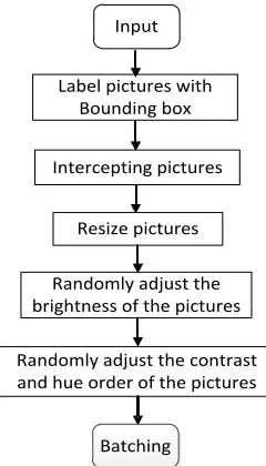
The image size was set to 180*200. In addition, brightness, contrast and hue of the images were randomly adjusted to reduce the impacts of irrelevant factors. Finally, N images were randomly selected from the training set for batch training. The preprocessing flowchart is shown in Figure 4.

Randomly adjust the contrast and hue order of the pictures

Randomly adjust the brightness of the pictures

Resize pictures Intercepting pictures

Label pictures with Bounding box

Input

Batching

Figure 4. Image Preprocessing Flowchart.

Experimental Result Analysis

This experiment explored the impacts of parameter setting, number of convolutional layers and moving average model on the model recognition accuracy. Specifically, Network 1, 2 and 3 were trained to obtain the impacts of parameter setting, number of convolutional layers and moving average model on the recognition accuracy respectively.

Impacts of Parameter Setting on the Model Accuracy. Due to the various parameters of deep learning, we tuned the learning rate, decay rate and momentum of Model 3 to explore their impacts on the recognition accuracy. Learning rate is a parameter that is widely used to minimize model errors. Decay rate can be used to adjust the impact of model complexity on the loss function. Momentum can accelerate the convergence of the model and batch size can effectively improve the model prediction accuracy.

Table 3. Impacts of Parameter Setting on the Model Accuracy.

Learning rate base

Learning rate decay

Moving average decay

Accuracy of training(%)

Accuracy of

testing(%) Batching

NET THREE

0.01 0.001 0.9 100 50.3 30

0.01 0.005 0.9 100 50.3 30

0.01 0.005 0.92 100 50.3 30

0.01 0.005 0.95 100 50.1 30

0.008 0.005 0.92 100 50.1 30

0.02 0.005 0.92 100 50.7 30

0.01 0.005 0.92 100 52 60

0.01 0.005 0.92 100 52.2 100

0.01 0.005 0.92 99 52.6 200

rate and the momentum remained unchanged (0.005 and 0.92 separately), the model accuracy varied with the changes in learning rate (0.01, 0.008 and 0.02). The model achieved its highest accuracy when the learning rate was 0.02 in that case. Therefore, the error rate could be reduced by changing the learning rate. When the learning rate, decay rate and momentum were set to 0.01, 0.005 and 0.92 respectively, the highest model accuracy occurred at the batching=200. Therefore, the more data in the dataset will result in better fitting effects and higher accuracy.

Impacts of the Number of Convolutional Layers on the Model Accuracy. Since convolutional layers are responsible for local feature extraction in deep learning, the model complexity and model accuracy are determined by the number of convolutional layers. Too many layers tend to increase the difficulties in model fitting while too few layers may cause insufficient feature extraction and eventually reduce the recognition accuracy. Therefore, the number of convolutional layers has a direct and decisive impact on the quality of the model.

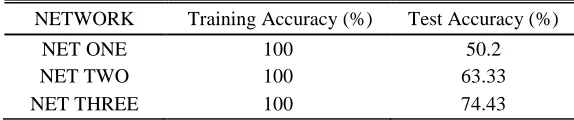
Table 4. Impacts of the Number of Convolutional Layers and Moving Average Model on the Accuracy.

NETWORK Training Accuracy (%) Test Accuracy (%)

NET ONE 100 50.2

NET TWO 100 63.33

NET THREE 100 74.43

Under the same parameters, Network 1 has 4 convolutional layers while Network 2 has 7 convolutional layers. It can be seen from Table 2 that the model trained by Network 2 has a higher accuracy than that trained by Network 1. Therefore, increase in the number of convolutional layers may abstract the image features extracted and enhance the model robustness.

Impacts of Moving Average Model on the Model Accuracy. Moving average model can enhance the model robustness. When the neural network is trained by stochastic gradient descent algorithm, differences between the parameters before and after update are controlled by regulating the decay rate of the moving average model. In this way, the parameter changes are mitigated and the impacts of sudden changes in local variables are effectively prevented.

In the control experiment, Network 2 has no moving average model while Network 3 has a moving average model. It can be seen from Table 3 that moving average model controls the model update velocity and prevents the impacts of sudden changes in local variables, thereby effectively improving the recognition accuracy.

Conclusion

This paper proposes a CNN-based vehicle model recognition method and explores the impacts of parameter setting, number of convolutional layers and moving average model on the recognition accuracy through experiments. The experimental results show that the recognition accuracy reaches 74.3%. In addition, the model is properly adjusted and improved. The method proposed, which has certain feasibility and use value, provides reference and experience for vehicle model recognition.

Acknowledgements

This work is financially supported by the Natural Science Foundation of Beijing (4174091), Research Funds for Education Committee of Beijing (KM201711232013), Key Research Project of Beijing Natural Science Foundation (Z16002) and 2018Talent-Development Quality Enhancement Project of BISTU (5111823402).

References

[1]Ju Zhang, Ting Zhang, Zheng-lingYang, Vehicle model recognition method based on deep convolutional, Transducer and Microsystem Technologies (2016) 11-0019-04.