14th International Conference on Wireless Communications, Networking and Mobile Computing (WiCOM 2018) ISBN: 978-1-60595-578-0
A Novel Selection and Matching of Patterns Model for Traffic
Prediction in Wireless Network
Qiangqiang Shen and Luyu Gao
ABSTRACT
Data mining techniques are becoming increasing popular and important in the big data era. Among them, frequent patterns mining technique has matured, with this technique, we can obtain the association rules to predict the data in cellular network. Existing research mainly focus on the frequent item sets mining, rarely involves in the time series and FPM algorithm usually used user-defined minimum support in various training datasets, which is rigorous, may influence the number of the frequent patterns and fail to select the reasonable patterns. Moreover, traditional association rules mining only relies on single evaluation criterion such as confidence or support, which leads to select unsound rules. This paper introduces an optimized frequent pattern mining algorithm, improving the setting of support in the process of mining frequent sequences and presenting a new evaluation criterion for the candidate patterns. Experiments were conducted to select appropriate parameters, support and evaluation criterion. Furthermore, we apply the above conclusion to the cellular flow data prediction, and compare the runtime, matching rate, RMSE and MAPE of proposed algorithms with those of improved Markov algorithm to examine the effectiveness of algorithm.
KEYWORDS: FP-Tree; Rules evaluation; Data prediction; Wireless Cellular Network
1. INTRODUCTION
The rapid development of information technology industry leads to the explosive growth of information, and human has entered the big data era. Mining the useful information from mass data is becoming more urgent, data mining comes into being, which is the computational process of discovering patterns in large datasets, including frequent pattern (FP) mining, clustering and classification. As an important knowledge discovery technique, frequent pattern mining is utilized in various application fields such as trajectory patterns [1], social network mining [2] and traffic data analysis [3]. It can be divided into two categories, Apriori-like algorithms and non Apriori-like algorithms. For non Apriori-like algorithms, like FP-growth method, which can be applied to the flow data prediction. Specifically, rule generation can be seen as the first part of the prediction, while the second part is rule evaluation, candidate ARs (association rules) are selected according to the specific criterion.
Since the introduction of the FP-growth algorithm by Han et al. [4], the algorithm has led a new research for mining frequent patterns with the tree structure, which reduces database scanning times, while Apriori-like algorithm requires for multiple ___________________________
database scans. With regarding a large number of candidate item sets by FPM, Jun TAN [5] proposed an approach to mining closed frequent patterns for the sparse database; Luyu Gao [6] used the matrix-like frequent tree-pattern to store frequent patterns. In this paper, we modify the FP-tree structure to store the frequent sequence, which can store more patterns’ information. Considering a single minimum support could miss hidden information, Hu [7] proposed the CFP-growth with multiple minimum supports. In this paper, instead of previous user-defined support, we obtain the best selection proportional range of FPs in the total patterns by carrying out experiments, to help set up reasonable support value according to the above results.
The prediction performance is effected by the selection of association rules, and mining the effective rules from large ARs is vital to predict flow data accurately. Rule evaluation removes less useful rules to reduce mining time and search space in the phase of prediction. Candidate rules are selected according to user-defined criterion, so as to decide which rule will be sorted to predict current moment’s flow data. With regard to the rule evaluation, there exists several criteria. Bing Liu [8] compared confidence, support and creation time in turn among the generated rules to choose a high precedence rules, if the above three aspects’ value of two or more rules are the same, the one created first is chosen. Luyu Gao [6] considered the largest matrix as the matching pattern. Hernndez-Len [9] introduced the use of Netconf measure instead of support and confidence, then proposed an approach to rule ranking by combining Netconf with rules of a long length. Kiburm Song [10] applied cross-validation and aggregating rules to select ARs, defined a new concept of predict rate to measure algorithm prediction performance, removing redundant and low predictive power rules. In this paper, we propose a new comprehensive evaluation criterion of association rules including the predict rate to select the reliable rule.
In brief, the main contributions of this study are as follows: (1) The number of frequent patterns could affect runtime of prediction and the accuracy of algorithm, we can get better performance by setting proportion of frequent patterns in the total pattern sets. (2) Introduced a method of rule-scoring, selecting ARs from candidate rules by a comprehensive criterion of confidence, prediction rate and length. Experiments revealed the appropriate combination of criteria could improve prediction performance. (3) Proposed a novel concept, prefix-path length, and analyzed its effect for prediction performance. Experiments show that with the prefix-path length increasing, algorithm shows higher prediction power and more time consuming. (4) Experiments have been conducted to compare the performance of proposed approach against Markov algorithm. The result shows that optimized FPM algorithm enhances the prediction accuracy.
2. PATTERN MINING AND THE CONSTRUCTION OF FP-TREE
2.1 DATASET PROCESSING
In this paper, we use the cellular network data of Nanjing from 2014.6.16 to 2014.6.30 for the experiment, which contains 15 days’ and 449 base stations’ data, is divided into 10 days for training data and 5 days for testing data. Since the minimum time granularity of raw data is 5 minutes, we accumulate the flow data to get 3 datasets whose time granularity are 30min, 45min, and 1hour respectively. Then we sort the flow data in order, and grade the datasets to disperse serial data from 1 to 5, 1 denotes the least value and 5 denotes highest value. Thus, we take the above discrete data as initial data DB, first ten days of which, DT, is seen as training data, the remaining data is test data.
2.2 THE PROCESS OF MINING FREQUENT SERIES PATTERNS
Consider DT as input data to generate all the patterns, DT is seen as a two- dimensional matrix, including two dimensions, time and locations (base station), containing the flow data of a time and a location, we extract all preliminary transactions of defined size by using the sliding window. Specifically, for the window size, we adopt a time-first scheme, expand the time dimension m from 5 to 12(a short period of time cannot extract the traffic variation rule), and then expand the base station n from 1 to 3. Each slide of the window produces a new transaction, each scan of the dataset produces a set of transactions of equal size. Then we obtain all the transactions’ groups. For each transaction (also called pattern) N, N can be seen as frequent pattern with the two requirements: 1. pattern N’s prefix sequence without the last item is FP, for example, if it’s known that [1,2,2] isn’t FP,[1,2,2,3] can’t be FP; 2.sup(N)≥ minSup(minimum support, the user-defined threshold), then N is said to be a FP. Therefore, we can get all the FPs. More than anything, considering that all the transactions are time series patterns, for example, pattern [2,3,1,2] is totally different from pattern [2,3,2,1]. Thus, frequent patterns we gain can get association rules directly, actually. For example, if [2,3,1,2] is a FP, [2,3,1]→[2] is an association rule. Specifically, mining FPs from transaction groups is shown Algorithm 1. As a result, we can pick out all the qualified series patterns, which are included in several sets, the same set contains the frequent series patterns of the same size.
Algorithm 1 Mining Frequent patterns Input: DT; support threshold minSup
Output: Rules, FP-Tree of various size 1: Create transset2n m* as the null list;
2: Scan DT to find out all the transactions sets TSn m* , which size ranges from 1*5 to 2*12;
3: for each transaction T in TSn m* do
4: Create transset1n m* as the null list;
5: ifm is5 then
6: Add T to transset1n m* (means T meets the condition) 7: elseif T’s prefix-path is frequent then
9: end if
10:end if
11: for each transaction T in transset1n m* do
12: if T isn’t included in transset2n m* and sup( )T minSup then
13: Add T and its support totransset2n m*
14: end if
15: end for
16: call the createTree(transset2n m* ) to get FP-Tree, Headertable
17: Create a list of rules to store each size’s transset2n m* , a list of tree to store each size’s FP-Tree and a list of Headertable sets to store each size’s Headertable;
18: returnrules, tree sets, Headertable sets
2.3 THE CONSTRUCTION OF FP-TREE
We can construct the corresponding FP-tree using above FPs’ sets, unlike storing the transactions into the submatrix [6], which just contains the information of item’s order. In this paper, the tree structure we used stores more pattern’s information, in which each node contains 5 values: node’s name, count (the number of the same prefix path and depth), node’s link (to link the same item in the different path), parent (to link the current node’s previous node), children (the child nodes associated with this node).
FP-tree is filled according to the algorithm shown Fig.2, data_Dict denotes a dictionary of transaction with the same size, whose value is the number of transactions, denoted by count. The algorithm calls the updateTree function to grow the FP-tree.
Algorithm 2 Modified FP-Tree construction Input: data_Dict;
Output: Headertable; Tree
1: Create the root node of FP-Tree;
2: for each transaction Tdata Dict_ do
3: Create the Headertable of each item, update its occurrence-frequency; 4: Expand the Headertable to store the first occurrence’s pointer of each item; 5: call updateTree(T.keys, Tree, Headertable, count)
6: return Tree, Headertable;
7: function updataTree(items, tree, Headertable, count) 8:if the first element E of items in tree then
9: sup(E)=sup(E)+count; 10:else
11: Create a new child node E of tree with sup(E)=count; 12: if the pointer p of E in the Headertable is null then
13: P is linked to E of the tree;
14: elseUpdate the Headertable to make sure nodelink can traverse each instance of the same item in the tree;
15: end if
16: end if
17: if the length of item >1 then
18: updateTree( items[1::], Tree.children, Headertable,count); 19: end if
2.4 SETTINGAPPROPRIATESUPPORTVALUE
Support threshold is an important parameter for the process of mining FPs. If the threshold is too large, the number of frequent patterns that meet condition above mentioned is poor, which will narrow down the choices of association rules in the prediction. If the threshold is too small, it will generate excess frequent patterns, which could be time consuming. We carried out the experiments by setting different ratio of frequent patterns in the total patterns to compare the prediction results. Different ratio of frequent patterns corresponddifferent support values, therefore we change ratio of frequent patterns, that means, change support to control the pattern mining. The procedural details of experiments are described in the section 4.
3. PATTERN MATCHING AND RULE SELECTION
3.1 SEVERAL CRITERIA OF RULE EVALUATION
Definition 1. (confidence, prefix-path) Supposed a series pattern defined by P on the form of A=>B, B is a single item, confidence is the ratio of the pattern P’s support over the pattern A’s support, called conf(P). The association rule is an implication of A=>B. Prefix-path is a path whose child node is current item. For example, for the rule A=>B, A (left-hand side) is the prefix-path of B (right-hand side).
Definition2.(prediction rate, support) Support is the number of a pattern P (or transaction) in all the transactions. After obtain all the FPs (initial candidate rule set), we can measure the prediction power of a frequent pattern by calculating the prediction rate. First, we divide the training dataset into k equal-length folds along base station dimension and produce k loops using k equal-length folds [10], in each loop i, we create inner training set TRi with (k-1) folds and inner testing set TEi with 1 fold. For each candidate pattern P, we calculate the ratio pi of the P’s support in TRi to patterns’ amount of same size in TRi and the ratio qi of the Q’s (P’s prefix-path) support in TEi to patterns’ amount of same size in TEi. We perform the same operation in each loop, add up all the pi and qi, then calculate average value to acquire prediction rate of P.
3.2 THE PROCESS OF PATTERN-MATCHING AND PREDICTION
Algorithm 3. Among them, the rules, conf, prediction rate, tree sets in the algorithm are all lists, BSs and TSs mean base stations and time slots, the first element of which stores the various attributes of rules which is 1 × 5, the second stores 1 × 6-size rules’ attributes, and so forth. Pc, pp and pl indicate the weightof confidence, prediction rate and length in the evaluation criterion.
3.3 EVALUATINGFORECASTACCURACY
We use MAPE, RMSE and matching rate to measure the quality of model. Matching rate, which measure the accuracy of prediction; MAPE is mean absolute error, and RMSE is root mean squared error, which both measure the average magnitude of the errors and are calculated as follows:
1 1 n
j j
j
MAPE y y
n
(1)2 1 1 ( ) n j j j
RMSE y y
n
(2)In this paper, we choose improved Markov method as the baseline algorithm, the basic idea of which is: for the sequential data pattern, we first adopt k-order Markov
method, and if the prefix-path isn’t exist in history path, then we calculate the lower order probability in order. At last we can get one or several matching-paths, then we calculate and compare path’s probability [11] to get the prediction value.
Algorithm 3 Modified FP-Tree construction
Input:DB,rules, Headertable sets,confidence, prediction rate, tree sets
Output: predictResult
1: Create predictResult as the null list; 2: for each time slot to be predicted do
3: Let rowspan=0; (rowspan denotes by rs)
4: Let prefixDat be time slots’ data before the current time slot of all the BSs; 5: whileDB[rs:rs+1,:] isn’t null do
6: for BSs’ amount of the prefix-path do
7: for TSs’ amount of the prefix-pathdo
8:candiset=prefixDat[rs:rs+n,-m:];
9:Let myFPtree and myHeadertable be tree and Headertable of candiset’s size in sets;
10: Search the path whose parent path matches candiset , create a list predicPath to store above mentioned path;
11: for each currPath in predicPath do
12: Obtain confidence, prediction rate, size of each currPath, calculate the score, score=conf*pc+length*pl+predictionrate*pp
13: Select rule with max score as selection 14:predictResult+=selection[-1]
15: rowspan=length(selection[-1]) 16: end while
17: end for
4. EXPERIMENTS
4.1 SELECT EFFECTIVE PARAMETERS
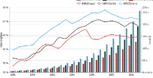
[image:7.612.174.424.251.379.2]All experiments were performed on a laptop with an Intel Core i3-370 M CPU (2.4 GHz) .All programs were coded in Python in Windows 8.1(64-bit), and run on the Microsoft. Firstly, we select appropriate proportion of frequent patterns according to the prediction performance. The experiments were conducted by setting different support, to each of these support values there corresponds a ratio of FP in the total patterns. For example, if the number of total preliminary transactions is 1000000, and we define the share of FPs is 20%, it means the number of FPs is 200000 and we should select the occurrence’s frequency of 200000th of the total as the support value. Under the same share, dataset of different size should set different support value.
Figure 1. Matching rate and runtime of various proportion and datasets.
Considering that if the ratio of FPs is too low, we couldn’t find the frequent sequences which can match the current node’s prefix-path, pre-experiment shows if the ratio of FPs is lower than 10%, the above-mentioned problem occurs frequently. Therefore, the ratio we set is start from 10%. For different time granularity, in Figure 1, the matching rate increases firstly and then decreases slightly as the ratio increases, while runtime increases gradually. In Figure 2, RMSE and MAPE decrease gradually and then increased slightly as the ratio increases. In general, experiments show that if proportion of FPs is between 20% and 25%, the prediction performance is superior to others, which should be an appropriate range. In addition, the prediction performance, decreases with the time granularity become bigger. If time granularity is smaller, the size of train sets is bigger, and leads to the larger number of the preliminary transactions, more accurate results and more time consumption.
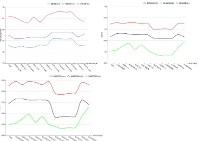
Figure 2. RMSE and MAPE of various proportion and datasets.
In Figure 3, with the change of evaluation criterion, matching rate, RMSE and MAPE would be changed slightly. Experiments show that when the weight of confidence is 0.3, the performance is better. Among the several experiments with fixed confidence’s weight, the performance indicates that 0.3:0.4:0.4 is the best ratio to measure the candidate rules. In addition, same as the conclusion above, when time granularity is smaller, the prediction performance is better.
Figure 3. Matching rate, RMSE and MAPE of various evaluation criteria and datasets.
4.2THEEFFECTIVENESSOFPROPOSEDALGORITHM
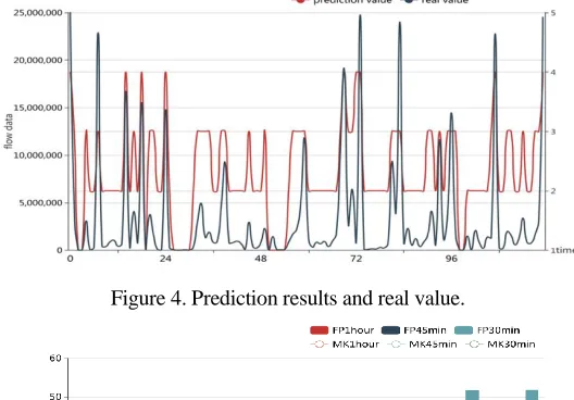
[image:8.612.105.503.306.589.2]Figure 4. Prediction results and real value.
Figure 5. Running time of various prefix-path length in two algorithms
In Figure 5 and 6, we choose 1 hour as time granularity, comparing the prediction performance and runtime of the improved Markov algorithm and modified FPM algorithm. The results show that prediction performance of proposed algorithm is better than those of Markov in various path length. With the increase of prefix-path length, modified FPM algorithm shows better performance and the improved Markov algorithm’s prediction ability is getting worse. However, the runtime of various prefix-path length for FP algorithm is longer than those of Markov. In addition, under the same conditions, for these two algorithms, matching rate of 30min’s data is better than those of 1hour’s and 45min’s, and RMSE and MAPE of proposed algorithm is lower than those of Markov in various prefix-path length. In general, the proposed algorithm shows good prediction performance.
5. CONCLUSION
This paper proposed the modified FP algorithm for mining FPs that used the modified FP-tree to store the candidate rules, and also proposed a comprehensive criterion to score the association rules. To show the effectiveness of the proposed algorithm, experiments were conducted on several datasets to select appropriate parameters at first, and then we applied above parameters to the data prediction. By compared the result with Markov algorithm, the results show that FP algorithm has less error and higher stability than improved Markov algorithm. In the future work, we will try to classify the base stations, then apply the above modified algorithm for mining frequent patterns of base station of the same class to increase the accuracy.
ACKNOWLEDGMENT
This work is supported by the National Science Foundation of China (NSFC)
under grant 61771065, 61571054 and 61631005.
REFERENCES
1. L. Wang, K. Hu and X. Yan: Mining frequent trajectory pattern based on vague space partition. Knowl. Based Syst.50,100–111(2013).
2. S.K. Tanbeer, C.K. Leung and J.J. Cameron: Interactive mining of strong friends from social networks and its applications in e-commerce. Journal of Organizational Computing and Electronic Commerce.24(2-3),157–173, 2014.
3. G. Fang, Z. Deng and H. Ma: Network traffic monitoring based on mining frequent patterns. Fuzzy Syst. Knowl. Disc. 7, 571–575(2009)
4. J. Han, J. Pei and Y. Yin: Mining frequent patterns without candidate generation. the 2000 ACM SIGMOD International Conference on Management of Data. 1– 12(2000)
5. Jun TAN, Yingyong BU: An Efficient Close Frequent Pattern Mining Algorithm Second International Conference on Intelligent Computation Technology and Au tomation IEEE. (2009). 6. Luyu Gao, Xing Zhang and Wenbo Wang: Spatiotemporal Traffic Modeling based on Frequent
Pattern Mining in Wireless Cellular Network. The 10th IEEE International conference on Cyber, Physical and Social computing.60– 67(2017).
8. B. Liu, W. Hsu and Y. Ma: Integrating classification and association rule mining. The 4th international conference on knowledge discovery and data mining.80–86.
9. R. Hernndez-Len, J. Hernndez-Palancar and J.F. Martnez-Trinidad: Studying netconf in hybrid rule ordering strategies for associative classification. The 6th Mexican conference on pattern recognition. 51–60.
10. Kiburm Song, Kichun Lee: Predictability-based collective class association rule mining. Expert Systems With Applications.79, 1–7(2017).